EVLA 6cmWideband Tutorial SN2010FZ CASA 4.2: Difference between revisions
| (4 intermediate revisions by the same user not shown) | |||
| Line 6: | Line 6: | ||
This article describes the calibration and imaging of a single-pointing 6-cm EVLA wideband continuum dataset of the galaxy NGC2967 (UGC5180) which was the location of the supernova candidate SN2010FZ. No supernova was detected in this observation, but the galactic continuum emission from this face-on spiral is nicely imaged. The data were taken in with 1024 MHz of bandwidth in each of two widely spaced basebands (each comprised of 8 128-MHz spectral windows), spanning 4.5 to 7.5 GHz. We will use wideband imaging techniques in this tutorial. | This article describes the calibration and imaging of a single-pointing 6-cm EVLA wideband continuum dataset of the galaxy NGC2967 (UGC5180) which was the location of the supernova candidate SN2010FZ. No supernova was detected in this observation, but the galactic continuum emission from this face-on spiral is nicely imaged. The data were taken in with 1024 MHz of bandwidth in each of two widely spaced basebands (each comprised of 8 128-MHz spectral windows), spanning 4.5 to 7.5 GHz. We will use wideband imaging techniques in this tutorial. | ||
This is a more advanced tutorial, and if you are a relative novice (and <em>particularly</em> for EVLA continuum calibration and imaging), it is <em>strongly</em> recommended that you start with the [[EVLA Continuum Tutorial 3C391]] (at least read it through) before tackling this dataset. We will not include basic information on CASA processing in this tutorial. | This is a more advanced tutorial, and if you are a relative novice (and <em>particularly</em> for EVLA continuum calibration and imaging), it is <em>strongly</em> recommended that you start with the [[EVLA Continuum Tutorial 3C391 CASA 4.2]] (at least read it through) before tackling this dataset. We will not include basic information on CASA processing in this tutorial. | ||
From the [http://casaguides.nrao.edu MainPage] of this guide you can find helpful information: | From the [http://casaguides.nrao.edu MainPage] of this guide you can find helpful information: | ||
| Line 576: | Line 576: | ||
Note that there are significant position corrections for a number of the antennas. | Note that there are significant position corrections for a number of the antennas. | ||
In CASA 4.1, we now have the option to use {{gencal}} to create a calibration table containing the gain curves for the antennas. Although you can still use the <tt>gaincurve=True</tt> option in each task, we will make use of this new feature (note that the <tt>gaincurve=True</tt> will be phased out in future CASA releases): | In CASA 4.1 and later, we now have the option to use {{gencal}} to create a calibration table containing the gain curves for the antennas. Although you can still use the <tt>gaincurve=True</tt> option in each task, we will make use of this new feature (note that the <tt>gaincurve=True</tt> will be phased out in future CASA releases): | ||
<source lang="python"> | <source lang="python"> | ||
# In CASA | # In CASA | ||
| Line 1,353: | Line 1,353: | ||
For more information on using {{clean}}, in particular on using the interactive GUI, see | For more information on using {{clean}}, in particular on using the interactive GUI, see | ||
[[ | [[EVLA_Continuum_Tutorial_3C391_CASA_4.2#Initial Imaging]]. WARNING: In CASA 4.0 the GUI interface for clean | ||
and the viewer has changed slightly. Some of the screenshots shown below may differ slightly | and the viewer has changed slightly. Some of the screenshots shown below may differ slightly | ||
from what you see. | from what you see. | ||
NOTE: If you are pressed for time, then you might want to jump ahead to | NOTE: If you are pressed for time, then you might want to jump ahead to | ||
[[ | [[EVLA_6cmWideband_Tutorial_SN2010FZ_CASA_4.2#Cleaning_the_lower_baseband_using_two_MFS_Taylor_terms]] | ||
and while it is cleaning you can read the other Imaging descriptions. | and while it is cleaning you can read the other Imaging descriptions. | ||
| Line 1,602: | Line 1,602: | ||
psfmode='clark',imsize=[1280,1280],cell=['3.0arcsec'],stokes='I', \ | psfmode='clark',imsize=[1280,1280],cell=['3.0arcsec'],stokes='I', \ | ||
imagermode='csclean', cyclefactor=4.5, \ | imagermode='csclean', cyclefactor=4.5, \ | ||
mask='imgSN2010FZ10s_spw0to11_mfs2_clean1280.mask', \ | |||
weighting='briggs',robust=0.5,interactive=True) | weighting='briggs',robust=0.5,interactive=True) | ||
</source> | </source> | ||
This should start cleaning from where our previous non-interactive clean left off. | |||
<b>Note for 4.2.0:</b> In this case we have specified <tt>mask='imgSN2010FZ10s_spw0to11_mfs2_clean1280.mask'</tt> explicitly due to a bug where it will not otherwise allow you to edit the mask interactively. | |||
You might find a few more sources revealed in the outer parts of the image, and also more | You might find a few more sources revealed in the outer parts of the image, and also more | ||
| Line 1,620: | Line 1,624: | ||
</source> | </source> | ||
The final rms achieved here is 8. | The final rms achieved here is 8.7 uJy; slightly better. | ||
== Analyzing the image == | == Analyzing the image == | ||
| Line 1,644: | Line 1,648: | ||
The output gives: | The output gives: | ||
<pre> | <pre> | ||
Residual standard deviation = 8. | Residual standard deviation = 8.74577600158e-06 | ||
Image max flux = 0. | Image max flux = 0.00993354152888 | ||
Model total flux = 0. | Model total flux = 0.0341279412654 | ||
SN2010FZ peak S/N = | SN2010FZ peak S/N = 1135.81019307 | ||
SN2010FZ total S/N = | SN2010FZ total S/N = 3902.2199127 | ||
</pre> | </pre> | ||
These are the numbers I got in my run-through. You may get slightly different values depending on how deeply you cleaned. | |||
What do we expect? If we do {{listobs}} on this MS we see the scans: | What do we expect? If we do {{listobs}} on this MS we see the scans: | ||
| Line 1,804: | Line 1,809: | ||
# Use multi-scale clean by adding non-zero scales to the <tt>multiscale</tt> parameter. | # Use multi-scale clean by adding non-zero scales to the <tt>multiscale</tt> parameter. | ||
# Image the calibrators. What sort of dynamic range can you get on them? Is self-calibration needed (and if so what dynamic range do you get when you use it)? | # Image the calibrators. What sort of dynamic range can you get on them? Is self-calibration needed (and if so what dynamic range do you get when you use it)? | ||
# Try the <tt>testautoflag</tt> task (in 3.3.0 and later) to automatically flag RFI from the upper sideband. There is more information on running <tt>testautoflag</tt> in [http://casaguides.nrao.edu/index.php?title=EVLA_Wide-Band_Wide-Field_Imaging:_G55.7_3. | # Try the <tt>testautoflag</tt> task (in 3.3.0 and later) to automatically flag RFI from the upper sideband. There is more information on running <tt>testautoflag</tt> in [http://casaguides.nrao.edu/index.php?title=EVLA_Wide-Band_Wide-Field_Imaging:_G55.7_3.4 this tutorial]. | ||
== Credits == | == Credits == | ||
Latest revision as of 17:17, 6 February 2014
This is an Advanced EVLA data reduction tutorial that calibrates and images a 6-cm wide-band continuum dataset.
This casaguide is for Version 4.2.0 of CASA.
Overview
This article describes the calibration and imaging of a single-pointing 6-cm EVLA wideband continuum dataset of the galaxy NGC2967 (UGC5180) which was the location of the supernova candidate SN2010FZ. No supernova was detected in this observation, but the galactic continuum emission from this face-on spiral is nicely imaged. The data were taken in with 1024 MHz of bandwidth in each of two widely spaced basebands (each comprised of 8 128-MHz spectral windows), spanning 4.5 to 7.5 GHz. We will use wideband imaging techniques in this tutorial.
This is a more advanced tutorial, and if you are a relative novice (and particularly for EVLA continuum calibration and imaging), it is strongly recommended that you start with the EVLA Continuum Tutorial 3C391 CASA 4.2 (at least read it through) before tackling this dataset. We will not include basic information on CASA processing in this tutorial.
From the MainPage of this guide you can find helpful information:
- What is CASA?
- Getting Started in CASA
- CASA Reference Manuals
- Hints, Tips, & Tricks
- AIPS-to-CASA Cheat Sheet
In this tutorial we will be invoking the tasks as function calls. You can cut and paste these to your casapy session. We also recommend that you copy all the commands you use, with any relevant commentary, to a text file. This is good practice when tackling large datasets. If you wish, you can use the Script Extractor to create a file with the tutorial commands, which can subsequently be edited as desired.
Occasionally we will be setting Python variables (e.g. as lists for flags) outside the function call so make sure you set those before running the task command. Note that when you call a CASA task as a function the task parameters you do not set in the function call (assuming there is at least one) will be set to their defaults, and will not use values you set in previous calls or outside the call. See Getting_Started_in_CASA#Task_Execution for more on calling tasks and setting parameters in the scripting interface.
NOTE: If you find that the figures on the right margin of the browser window overlap the text too much and make reading difficult, go ahead and widen the browser window.
Obtaining the Data
The data for this tutorial were taken with the EVLA under program AS1015 as the scheduling block (SB) AS1015_sb1658169_1.55388.89474846065, and was run on 2010-07-11 from 21:28 to 22:28 UT (size 37.74GB).
The data can be directly downloaded from http://casa.nrao.edu/Data/EVLA/SN2010FZ/SN2010FZ_10s.ms.tar.gz (dataset size: 2.9 GB). For example, in you Linux terminal:
wget http://casa.nrao.edu/Data/EVLA/SN2010FZ/SN2010FZ_10s.ms.tar.gz
Your first step will be to unzip and untar the file in a terminal, before you start CASA:
tar -xzvf SN2010FZ_10s.ms.tar.gz
If you are brave enough, you can also get the data straight from the EVLA archive. Go to the NRAO Science Data Archive, and search for project **AS1015**. Then select the AS1015_sb1658169_1.55388.89474846065 dataset and choose to apply the online flags (check box "Apply flags generated during observing") and time-averaging of 10 seconds. (The data were taken in D-configuration [max baselines 1km], so one can safely average to 3s or even 10s to reduce dataset size.) Also select the tar option. This will create a file equivalent to what is used at the workshop.
Starting CASA
To start CASA, type:
casapy
This will run a script to initialize CASA, setting paths appropriately. It will also start writing to a file called ipython.log, which will contain a record of all the text you enter at the CASA prompt.
A logger window will also appear; note that you can rescale this window or change the font size as desired (the latter is under "View"). The messages which are printed to the logger are also saved to a file called casalog.py, and any previous version of casalog.py which may have been present is moved to a backup version with a date stamp. Note that this does not happen for any previous versions of ipython.log, so if you wish to save one, be sure to rename it before restarting CASA.
Examining the MS
We use listobs to summarize our MS:
# In CASA
listobs('SN2010FZ_10s.ms')
In the logger you should see:
##########################################
##### Begin Task: listobs            #####

================================================================================
           MeasurementSet Name:  SN2010FZ_10s.ms      MS Version 2
================================================================================
   Observer: Dr. Alicia M. Soderberg     Project: T.B.D.
Observation: EVLA
Data records: 1570726       Total integration time = 3359 seconds
   Observed from   11-Jul-2010/21:30:44.0   to   11-Jul-2010/22:26:43.0 (UTC)

   ObservationID = 0         ArrayID = 0
  Date        Timerange (UTC)          Scan  FldId FieldName           nRows   Int(s)   SpwIds      ScanIntent
  11-Jul-2010/21:30:44.0 - 21:30:52.0     2      0 J0925+0019          404    6.43     [0, 1]                      CALIBRATE_PHASE#UNSPECIFIED
              21:31:02.0 - 21:32:22.0     3      0 J0925+0019          5062   9.68     [0, 1]                      CALIBRATE_PHASE#UNSPECIFIED
              21:32:32.0 - 21:33:52.0     4      0 J0925+0019          6277   9.91     [0, 1]                      CALIBRATE_PHASE#UNSPECIFIED
              21:34:02.0 - 21:34:52.0     5      0 J0925+0019          4148   9.96     [0, 1]                      CALIBRATE_PHASE#UNSPECIFIED
              21:35:02.0 - 21:35:51.5     6      0 J0925+0019          32640  9.44     [2, 3, 4, 5, 6, 7, 8, 9, 10, 11, 12, 13, 14, 15, 16, 17]CALIBRATE_PHASE#UNSPECIFIED
              21:36:01.0 - 21:38:20.5     7      0 J0925+0019          81600  9.93     [2, 3, 4, 5, 6, 7, 8, 9, 10, 11, 12, 13, 14, 15, 16, 17]CALIBRATE_PHASE#UNSPECIFIED
              21:38:44.0 - 21:39:51.0     9      1 SN2010FZ            43520  9.16     [2, 3, 4, 5, 6, 7, 8, 9, 10, 11, 12, 13, 14, 15, 16, 17]OBSERVE_TARGET#UNSPECIFIED
              21:40:01.0 - 21:41:20.5    10      1 SN2010FZ            48960  9.89     [2, 3, 4, 5, 6, 7, 8, 9, 10, 11, 12, 13, 14, 15, 16, 17]OBSERVE_TARGET#UNSPECIFIED
              21:41:30.0 - 21:42:50.0    11      1 SN2010FZ            48960  10       [2, 3, 4, 5, 6, 7, 8, 9, 10, 11, 12, 13, 14, 15, 16, 17]OBSERVE_TARGET#UNSPECIFIED
              21:43:00.0 - 21:44:20.0    12      1 SN2010FZ            48960  10       [2, 3, 4, 5, 6, 7, 8, 9, 10, 11, 12, 13, 14, 15, 16, 17]OBSERVE_TARGET#UNSPECIFIED
              21:44:30.0 - 21:45:50.0    13      1 SN2010FZ            48960  10       [2, 3, 4, 5, 6, 7, 8, 9, 10, 11, 12, 13, 14, 15, 16, 17]OBSERVE_TARGET#UNSPECIFIED
              21:46:00.0 - 21:47:19.5    14      1 SN2010FZ            48960  9.89     [2, 3, 4, 5, 6, 7, 8, 9, 10, 11, 12, 13, 14, 15, 16, 17]OBSERVE_TARGET#UNSPECIFIED
              21:47:29.0 - 21:47:49.0    15      1 SN2010FZ            16320  9.67     [2, 3, 4, 5, 6, 7, 8, 9, 10, 11, 12, 13, 14, 15, 16, 17]OBSERVE_TARGET#UNSPECIFIED
              21:48:12.0 - 21:49:18.5    16      0 J0925+0019          43520  9        [2, 3, 4, 5, 6, 7, 8, 9, 10, 11, 12, 13, 14, 15, 16, 17]CALIBRATE_PHASE#UNSPECIFIED
              21:49:42.0 - 21:50:49.0    17      1 SN2010FZ            43520  9.17     [2, 3, 4, 5, 6, 7, 8, 9, 10, 11, 12, 13, 14, 15, 16, 17]OBSERVE_TARGET#UNSPECIFIED
              21:50:59.0 - 21:52:19.0    18      1 SN2010FZ            48960  10       [2, 3, 4, 5, 6, 7, 8, 9, 10, 11, 12, 13, 14, 15, 16, 17]OBSERVE_TARGET#UNSPECIFIED
              21:52:29.0 - 21:53:48.5    19      1 SN2010FZ            48960  9.89     [2, 3, 4, 5, 6, 7, 8, 9, 10, 11, 12, 13, 14, 15, 16, 17]OBSERVE_TARGET#UNSPECIFIED
              21:53:58.0 - 21:55:18.0    20      1 SN2010FZ            48960  10       [2, 3, 4, 5, 6, 7, 8, 9, 10, 11, 12, 13, 14, 15, 16, 17]OBSERVE_TARGET#UNSPECIFIED
              21:55:28.0 - 21:56:48.0    21      1 SN2010FZ            48960  10       [2, 3, 4, 5, 6, 7, 8, 9, 10, 11, 12, 13, 14, 15, 16, 17]OBSERVE_TARGET#UNSPECIFIED
              21:56:58.0 - 21:58:18.0    22      1 SN2010FZ            48960  10       [2, 3, 4, 5, 6, 7, 8, 9, 10, 11, 12, 13, 14, 15, 16, 17]OBSERVE_TARGET#UNSPECIFIED
              21:58:28.0 - 21:58:47.5    23      1 SN2010FZ            16320  9.67     [2, 3, 4, 5, 6, 7, 8, 9, 10, 11, 12, 13, 14, 15, 16, 17]OBSERVE_TARGET#UNSPECIFIED
              21:59:10.5 - 22:00:17.0    24      0 J0925+0019          43520  8.99     [2, 3, 4, 5, 6, 7, 8, 9, 10, 11, 12, 13, 14, 15, 16, 17]CALIBRATE_PHASE#UNSPECIFIED
              22:00:39.5 - 22:01:47.0    25      1 SN2010FZ            43520  9.18     [2, 3, 4, 5, 6, 7, 8, 9, 10, 11, 12, 13, 14, 15, 16, 17]OBSERVE_TARGET#UNSPECIFIED
              22:01:57.0 - 22:03:17.0    26      1 SN2010FZ            48960  10       [2, 3, 4, 5, 6, 7, 8, 9, 10, 11, 12, 13, 14, 15, 16, 17]OBSERVE_TARGET#UNSPECIFIED
              22:03:27.0 - 22:04:47.0    27      1 SN2010FZ            48960  10       [2, 3, 4, 5, 6, 7, 8, 9, 10, 11, 12, 13, 14, 15, 16, 17]OBSERVE_TARGET#UNSPECIFIED
              22:04:57.0 - 22:06:16.5    28      1 SN2010FZ            48960  9.89     [2, 3, 4, 5, 6, 7, 8, 9, 10, 11, 12, 13, 14, 15, 16, 17]OBSERVE_TARGET#UNSPECIFIED
              22:06:26.0 - 22:07:46.0    29      1 SN2010FZ            48960  10       [2, 3, 4, 5, 6, 7, 8, 9, 10, 11, 12, 13, 14, 15, 16, 17]OBSERVE_TARGET#UNSPECIFIED
              22:07:56.0 - 22:09:16.0    30      1 SN2010FZ            48960  10       [2, 3, 4, 5, 6, 7, 8, 9, 10, 11, 12, 13, 14, 15, 16, 17]OBSERVE_TARGET#UNSPECIFIED
              22:09:26.0 - 22:09:45.5    31      1 SN2010FZ            16320  9.67     [2, 3, 4, 5, 6, 7, 8, 9, 10, 11, 12, 13, 14, 15, 16, 17]OBSERVE_TARGET#UNSPECIFIED
              22:10:08.0 - 22:11:15.5    32      0 J0925+0019          43520  9.13     [2, 3, 4, 5, 6, 7, 8, 9, 10, 11, 12, 13, 14, 15, 16, 17]CALIBRATE_PHASE#UNSPECIFIED
              22:11:38.0 - 22:12:45.5    33      1 SN2010FZ            43520  9.19     [2, 3, 4, 5, 6, 7, 8, 9, 10, 11, 12, 13, 14, 15, 16, 17]OBSERVE_TARGET#UNSPECIFIED
              22:12:55.0 - 22:14:15.0    34      1 SN2010FZ            48960  10       [2, 3, 4, 5, 6, 7, 8, 9, 10, 11, 12, 13, 14, 15, 16, 17]OBSERVE_TARGET#UNSPECIFIED
              22:14:25.0 - 22:15:45.0    35      1 SN2010FZ            48960  10       [2, 3, 4, 5, 6, 7, 8, 9, 10, 11, 12, 13, 14, 15, 16, 17]OBSERVE_TARGET#UNSPECIFIED
              22:15:55.0 - 22:17:15.0    36      1 SN2010FZ            48960  10       [2, 3, 4, 5, 6, 7, 8, 9, 10, 11, 12, 13, 14, 15, 16, 17]OBSERVE_TARGET#UNSPECIFIED
              22:17:25.0 - 22:18:44.5    37      1 SN2010FZ            48960  9.89     [2, 3, 4, 5, 6, 7, 8, 9, 10, 11, 12, 13, 14, 15, 16, 17]OBSERVE_TARGET#UNSPECIFIED
              22:18:54.0 - 22:20:14.0    38      1 SN2010FZ            48960  10       [2, 3, 4, 5, 6, 7, 8, 9, 10, 11, 12, 13, 14, 15, 16, 17]OBSERVE_TARGET#UNSPECIFIED
              22:20:24.0 - 22:20:43.5    39      1 SN2010FZ            16320  9.67     [2, 3, 4, 5, 6, 7, 8, 9, 10, 11, 12, 13, 14, 15, 16, 17]OBSERVE_TARGET#UNSPECIFIED
              22:21:06.0 - 22:22:13.5    40      0 J0925+0019          42690  9.15     [2, 3, 4, 5, 6, 7, 8, 9, 10, 11, 12, 13, 14, 15, 16, 17]CALIBRATE_PHASE#UNSPECIFIED
              22:25:13.0 - 22:25:13.0    42      2 3C286               1028   2.87     [2, 3, 4, 5, 6, 7, 8, 9, 10, 11, 12, 13, 14, 15, 16, 17]CALIBRATE_BANDPASS#UNSPECIFIED,CALIBRATE_AMPLI#UNSPECIFIED
              22:25:23.0 - 22:26:43.0    43      2 3C286               47757  9.6      [2, 3, 4, 5, 6, 7, 8, 9, 10, 11, 12, 13, 14, 15, 16, 17]CALIBRATE_BANDPASS#UNSPECIFIED,CALIBRATE_AMPLI#UNSPECIFIED
           (nVis = Total number of time/baseline visibilities per scan)
Fields: 3
  ID   Code Name                RA              Decl          Epoch   SrcId nVis
  0    D    J0925+0019          09:25:07.81503 +00.19.13.9334 J2000   0     303381
  1    NONE SN2010FZ            09:42:04.77000 +00.19.51.0000 J2000   1     1218560
  2    K    3C286               13:31:08.28798 +30.30.32.9589 J2000   2     48785
   (nVis = Total number of time/baseline visibilities per field)
Spectral Windows:  (18 unique spectral windows and 1 unique polarization setups)
  SpwID  #Chans Frame Ch1(MHz)    ChanWid(kHz)  TotBW(kHz)  Corrs
  0          64 TOPO  7686        2000          128000      RR  RL  LR  LL
  1          64 TOPO  7836        2000          128000      RR  RL  LR  LL
  2          64 TOPO  4488        2000          128000      RR  RL  LR  LL
  3          64 TOPO  4616        2000          128000      RR  RL  LR  LL
  4          64 TOPO  4744        2000          128000      RR  RL  LR  LL
  5          64 TOPO  4872        2000          128000      RR  RL  LR  LL
  6          64 TOPO  5000        2000          128000      RR  RL  LR  LL
  7          64 TOPO  5128        2000          128000      RR  RL  LR  LL
  8          64 TOPO  5256        2000          128000      RR  RL  LR  LL
  9          64 TOPO  5384        2000          128000      RR  RL  LR  LL
  10         64 TOPO  6488        2000          128000      RR  RL  LR  LL
  11         64 TOPO  6616        2000          128000      RR  RL  LR  LL
  12         64 TOPO  6744        2000          128000      RR  RL  LR  LL
  13         64 TOPO  6872        2000          128000      RR  RL  LR  LL
  14         64 TOPO  7000        2000          128000      RR  RL  LR  LL
  15         64 TOPO  7128        2000          128000      RR  RL  LR  LL
  16         64 TOPO  7256        2000          128000      RR  RL  LR  LL
  17         64 TOPO  7384        2000          128000      RR  RL  LR  LL
Sources: 50
  ID   Name                SpwId RestFreq(MHz)  SysVel(km/s)
  0    J0925+0019          0     -              -
  0    J0925+0019          1     -              -
  0    J0925+0019          2     -              -
  0    J0925+0019          3     -              -
  0    J0925+0019          4     -              -
  0    J0925+0019          5     -              -
  0    J0925+0019          6     -              -
  0    J0925+0019          7     -              -
  0    J0925+0019          8     -              -
  0    J0925+0019          9     -              -
  0    J0925+0019          10    -              -
  0    J0925+0019          11    -              -
  0    J0925+0019          12    -              -
  0    J0925+0019          13    -              -
  0    J0925+0019          14    -              -
  0    J0925+0019          15    -              -
  0    J0925+0019          16    -              -
  0    J0925+0019          17    -              -
  1    SN2010FZ            2     -              -
  1    SN2010FZ            3     -              -
  1    SN2010FZ            4     -              -
  1    SN2010FZ            5     -              -
  1    SN2010FZ            6     -              -
  1    SN2010FZ            7     -              -
  1    SN2010FZ            8     -              -
  1    SN2010FZ            9     -              -
  1    SN2010FZ            10    -              -
  1    SN2010FZ            11    -              -
  1    SN2010FZ            12    -              -
  1    SN2010FZ            13    -              -
  1    SN2010FZ            14    -              -
  1    SN2010FZ            15    -              -
  1    SN2010FZ            16    -              -
  1    SN2010FZ            17    -              -
  2    3C286               2     -              -
  2    3C286               3     -              -
  2    3C286               4     -              -
  2    3C286               5     -              -
  2    3C286               6     -              -
  2    3C286               7     -              -
  2    3C286               8     -              -
  2    3C286               9     -              -
  2    3C286               10    -              -
  2    3C286               11    -              -
  2    3C286               12    -              -
  2    3C286               13    -              -
  2    3C286               14    -              -
  2    3C286               15    -              -
  2    3C286               16    -              -
  2    3C286               17    -              -
Antennas: 27:
  ID   Name  Station   Diam.    Long.         Lat.
  0    ea01  W09       25.0 m   -107.37.25.2  +33.53.51.0
  1    ea02  E02       25.0 m   -107.37.04.4  +33.54.01.1
  2    ea03  E09       25.0 m   -107.36.45.1  +33.53.53.6
  3    ea04  W01       25.0 m   -107.37.05.9  +33.54.00.5
  4    ea05  W08       25.0 m   -107.37.21.6  +33.53.53.0
  5    ea06  N06       25.0 m   -107.37.06.9  +33.54.10.3
  6    ea08  N01       25.0 m   -107.37.06.0  +33.54.01.8
  7    ea09  E06       25.0 m   -107.36.55.6  +33.53.57.7
  8    ea10  N03       25.0 m   -107.37.06.3  +33.54.04.8
  9    ea11  E04       25.0 m   -107.37.00.8  +33.53.59.7
  10   ea12  E08       25.0 m   -107.36.48.9  +33.53.55.1
  11   ea13  N07       25.0 m   -107.37.07.2  +33.54.12.9
  12   ea14  E05       25.0 m   -107.36.58.4  +33.53.58.8
  13   ea15  W06       25.0 m   -107.37.15.6  +33.53.56.4
  14   ea16  W02       25.0 m   -107.37.07.5  +33.54.00.9
  15   ea17  W07       25.0 m   -107.37.18.4  +33.53.54.8
  16   ea18  N09       25.0 m   -107.37.07.8  +33.54.19.0
  17   ea19  W04       25.0 m   -107.37.10.8  +33.53.59.1
  18   ea20  N05       25.0 m   -107.37.06.7  +33.54.08.0
  19   ea21  E01       25.0 m   -107.37.05.7  +33.53.59.2
  20   ea22  N04       25.0 m   -107.37.06.5  +33.54.06.1
  21   ea23  E07       25.0 m   -107.36.52.4  +33.53.56.5
  22   ea24  W05       25.0 m   -107.37.13.0  +33.53.57.8
  23   ea25  N02       25.0 m   -107.37.06.2  +33.54.03.5
  24   ea26  W03       25.0 m   -107.37.08.9  +33.54.00.1
  25   ea27  E03       25.0 m   -107.37.02.8  +33.54.00.5
  26   ea28  N08       25.0 m   -107.37.07.5  +33.54.15.8

##### End Task: listobs              #####
##########################################
This task displays a lot of information about the MS. We can see that the observation was performed with the EVLA, for a total integration of 3359 seconds (1 hour). The number of data records (1570726) is equal to the number of baselines (N_antenna * [N_antenna - 1] / 2) X the number of integrations (observing time / time-average binning) X the number of spectral windows. For this observation, this is roughly 351 baselines (27X26/2) X 360 integrations (3600s total/10s avg) X 16 spectral windows = 2021760. Note that this is high by ~30%; this is because the archive already flagged bad data, and there are some scans which only have two (rather than 16) spectral windows present. Extra exercise: examine the MS using browsetable to see what a data record looks like (equivalent to a row, as displayed by this task).
The most useful parts of the listobs output are the scan, field, and spectral window listings.
From the spectral window information, we can see that there were a total of 18 (0 through 17) spectral windows in this dataset. The first two of these (0 and 1) were only used to help set up the correlator.
Looking at the scan listing, we can see that the first four scans which are present used only these spectral windows. These are referred to as "dummy scans". We will not be using these, since they often contain bad data.
The C-band data of interest is contained in scans 6-44 and spectral windows 2 to 17. Careful examination shows that scan 8 is missing but from the time ranges that the data has been merged into scan 7. This sort of correlator back-end data-capture issue was occasionally seen during 2010. Hopefully, it will not affect our data, but we should keep an eye out for problems with scan 7.
The field listing shows three sources:
- J0925+0019 (also referred to by its field ID, 0), which will serve as a calibrator for the visibility phases,
- SN2010FZ (1), our science target field, and
- 3C286 (2), which will serve as a calibrator for the visibility amplitudes, i.e., it is assumed to have a precisely known flux density; as well as the spectral bandpass.
Flagging the MS
The online flags, which are a record of known bad data produced by the EVLA online system, have already been applied by the archive as it generated the MS. However, it's good to have a sense of what was deleted in this process. A record of the flags is also stored in a separate table in the MS, called FLAG_CMD. (In fact, the information for this table is actually a subdirectory within the MS; you can see this by listing the contents of SN2010FZ_10s.ms.)
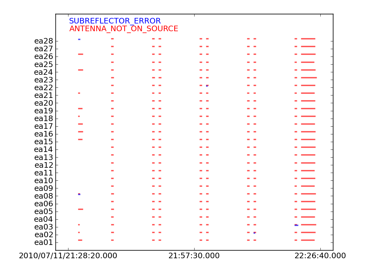
You can examine the commands stored in the FLAG_CMD table using flagcmd.
# In CASA
flagcmd(vis='SN2010FZ_10s.ms',inpmode='table',action='list')
These will go to the logger or terminal (they appear to go to the terminal now in 4.2).
You can also plot the commands stored in the FLAG_CMD table:
# In CASA
myrows = range(285)
flagcmd(vis='SN2010FZ_10s.ms',inpmode='table',action='plot',tablerows=myrows)
Note that we are only plotting the first 285 rows -- this is because the last few are from flagging zeros in the data (caused by correlator errors) and data which have been flagged due to antenna shadowing. Note that you can not do the tablerows selection and plot those too, you will just get lines at the bottom marked as "All" antennas for these flags.
This will bring up a matplotlib plotter. You can have it plot to a PNG file instead:
# In CASA
flagcmd(vis='SN2010FZ_10s.ms', inpmode='table', action='plot', tablerows=myrows,
        plotfile='PlotSN2010FZ_flagcmd_4.2.png')
The flags as plotted in the figure to the above right look normal. They are color-coded by REASON, and you see ANTENNA_NOT_ON_SOURCE flags between scans, and the occasional SUBREFLECTOR_ERROR flag also between scans (most likely after band changes when the subreflector rotates to pick up the new feed on the ring, some are slower than others). What you watch for here are long blocks of unexpected flags, which might be false alarms and cause you to flag too much data. In that case, look at the data itself in plotms (see below for examples) to decide whether or not to apply all flags.
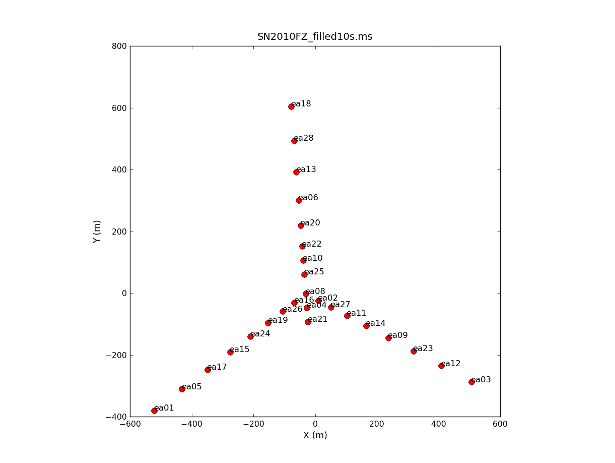
To plot up the antenna positions in the array:
# In CASA
plotants('SN2010FZ_10s.ms')
NOTE: if after this point (or any other) you get "table locks", which may occur erroneously and are sometimes triggered by plotting tasks, use clearstat to clear them:
# In CASA
clearstat
Now we examine the MS looking for bad data to flag. We will use plotms to bring up an interactive GUI that will display 2-D Y vs.X style line plots. NOTE: We do not recommend using the editing/flagging features of plotms. It is very easy to mess up your data this way. Also, to improve speed we will be restricting the scope of plotting so most box/flag operations would not get rid of all the bad data.
We will instead use plotms to identify bad data and then use flagcmd to flag it. This will also allow full scripting of the flagging, which is ultimately the best way to keep track of what's been deleted. Given the large dataset sizes now being generated, reproducibility is extremely important. Imaging spending a day flagging your data, then a disk error corrupts the MS. It's imperative that you have an automated way to regenerate your work. This is also why we encourage you to keep a running file with all the commands you use on a dataset.
NOTE: If you need an introduction to plotms, see:
- Data flagging with plotms
- Averaging data in plotms
- What's the difference between Antenna1 and Antenna2? Axis definitions in plotms
WARNING: The Flag ![]() button on the plotms GUI is close to other buttons you will be using, in particular the one that gets rid of boxes you have drawn. Be careful and don't hit the Flag button by mistake!
button on the plotms GUI is close to other buttons you will be using, in particular the one that gets rid of boxes you have drawn. Be careful and don't hit the Flag button by mistake!
As we found above, the useful spectral windows are 2-17. To get an idea of the data layout, plot a single baseline (ea01&ea02) and channel (31, for all spectral windows) versus time:
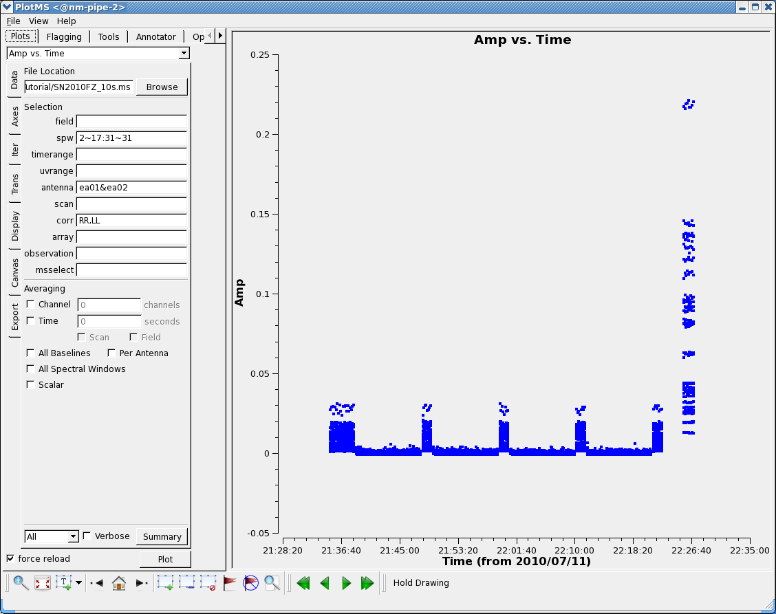
# In CASA
plotms(vis='SN2010FZ_10s.ms',field='',spw='2~17:31~31', \
       antenna='ea01&ea02',correlation='RR,LL',xaxis='time',yaxis='amp')
Here, we can see the alternating phase calibration and science target scans, as well as the (brighter) flux calibrator at the end of the observation. Feel free to play with ways to view, or color the data: for example, go to the "Display" left-hand tab, and choose "Colorize by: Field". You can also change the size of the plotted points, if they are too small to see easily, by setting "Unflagged Points Symbol" to "Custom" and increasing the number of pixels under "Style".
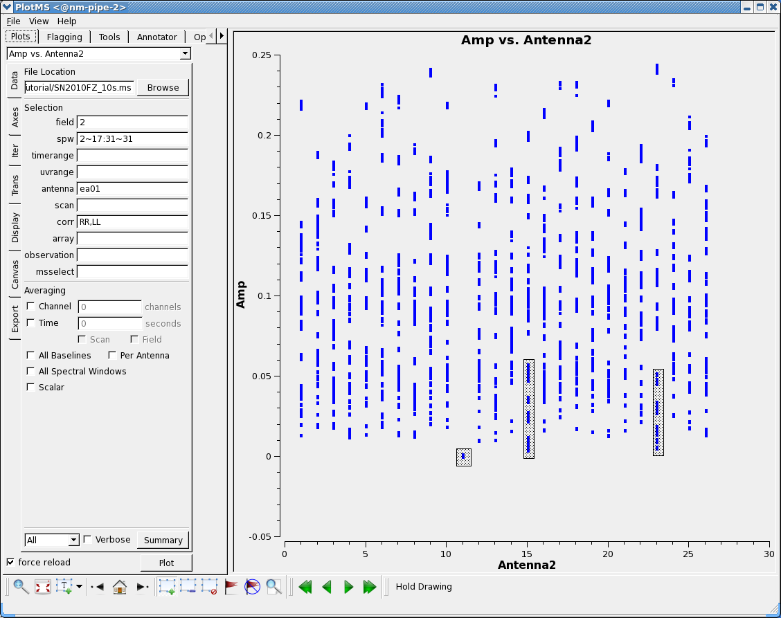
Look for bad antennas by picking the last field and plotting baselines versus antenna ea01:
# In CASA
plotms(vis='SN2010FZ_10s.ms',field='2',spw='2~17:31~31', \
       antenna='ea01',correlation='RR,LL',xaxis='antenna2',yaxis='amp')
You should be able to see that antenna 11 (= ea13) is bad (very low amplitude, it has no C-band receiver!) and that some of the spectral windows on 15 and 23 (ea17, ea25) are also on the low side. Boxing with the Mark Regions ![]() tool and using the Locate
tool and using the Locate ![]() tool will show in the logger that spw 10-17 are suspect for these antennas. (Note: you may also leave these in for now if you like; if this were truly a first pass through the data it is unlikely that they would be caught. Since this is a tutorial, and there is limited time for a second pass through the data, it's probably best to trust us and delete them now.)
tool will show in the logger that spw 10-17 are suspect for these antennas. (Note: you may also leave these in for now if you like; if this were truly a first pass through the data it is unlikely that they would be caught. Since this is a tutorial, and there is limited time for a second pass through the data, it's probably best to trust us and delete them now.)
Now look at the bandpass for ea02 - it is in the inner core and a prospective reference antenna. Exclude ea13 using negation (represented by "!") in the selection:
# In CASA
plotms(vis='SN2010FZ_10s.ms',field='2',spw='2~17', \
       antenna='ea02;!ea13',correlation='RR,LL',xaxis='frequency',yaxis='amp')
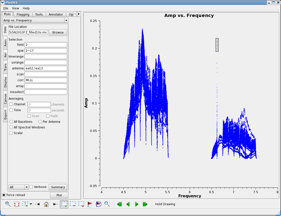
There is clearly less data for spw 11, and use of Locate shows spw 11 data only for ea02,ea03,04,08,09,11,12. We will later delete this incomplete spw. Note also the very strong RFI spike at 6614 MHz (spw 10 ch 63) with clear ringing contaminating both spw 10 and 11. There is also a tremendous roll-off in spw 10. We will drop these spectral window when we process the data.
We can also step through the baselines to our antenna using iteraxis:
# In CASA
plotms(vis='SN2010FZ_10s.ms',field='2',spw='2~17',antenna='ea02;!ea13', \
       correlation='RR,LL',xaxis='frequency',yaxis='amp',iteraxis='baseline')
and use the Next Iteration ![]() button to step through the baselines.
This will make it easier to isolate the bad antennas. Now plot the phases, iterating through baselines to ea02:
button to step through the baselines.
This will make it easier to isolate the bad antennas. Now plot the phases, iterating through baselines to ea02:
# In CASA
plotms(vis='SN2010FZ_10s.ms',field='2',spw='2~17',antenna='ea02;!ea13', \
       correlation='RR,LL',xaxis='frequency',yaxis='phase',iteraxis='baseline')
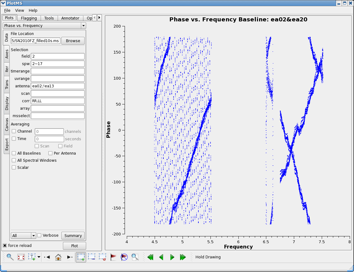
You see the slopes due to residual delays. Mostly a turn or less over a 128MHz subband, but there are some outliers. Step through to ea20. You see that there is a very large delay in RR (via locate) for the first baseband (spw 0~7). We will delete this (will also delete LL so there are no orphan polarization products, which would be ignored by clean in the imaging stage). Note ea17 and ea25 baselines drop close to zero in the middle of upper baseband (e.g. plot 'ea17&ea25') so we will delete these.
To carry out flagging, we again use flagcmd in the mode where it takes a list of command strings:
# In CASA
flaglist = ['antenna="ea13"',
            'antenna="ea17" spw="10~17"',
            'antenna="ea25" spw="10~17"',
            'antenna="ea20" spw="2~9"']
flagcmd(vis='SN2010FZ_10s.ms',inpmode='list',inpfile=flaglist,action='apply',flagbackup=True)
These commands will be carried out as well as being added to the FLAG_CMD table (marked as applied).
Plot the data again, now that is has been flagged:
# In CASA
plotms(vis='SN2010FZ_10s.ms',field='',spw='5:30~33',avgchannel='64', \
       antenna='ea01&ea02',correlation='RR,LL',xaxis='time',yaxis='amp')
plotms(vis='SN2010FZ_10s.ms',field='2',spw='2~17',antenna='ea02', \
       correlation='RR,LL',xaxis='frequency',yaxis='amp',scan='7~43')
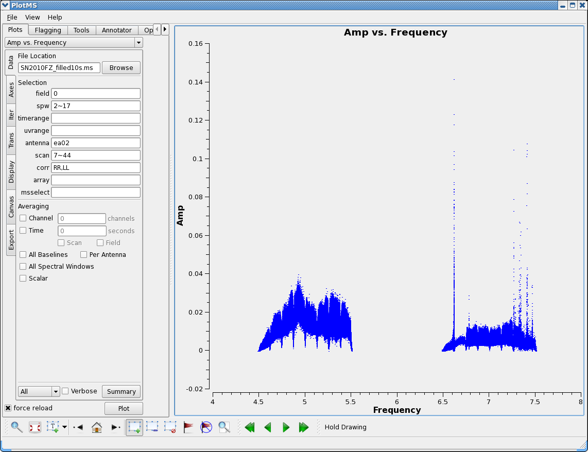
Now our phase calibrator - it is weaker, and we now start to really see the RFI:
# In CASA
plotms(vis='SN2010FZ_10s.ms',field='0',spw='2~17',antenna='ea02', \
       correlation='RR,LL',xaxis='frequency',yaxis='amp',scan='7~43')
Use the Zoom feature, Mark rectangles and use Locate to identify the frequency/channel of RFI. In particular, we note in our analysis:
- 6614MHz (spw 10 ch 63) super strong
- 6772-6778MHz (spw 12 ch 14-17)
- 7260-7264MHz (spw 16 ch 2-4)
- 7314-7340MHz (spw 16 ch 29-42)
- 7402-7418MHz (spw 17 ch 9-17)
- 7458-7466MHz (spw 17 ch 37-41)
- 7488MHz (spw 17 ch 52)
If you plot all antennas and avoid the band edges you see spw 16 and 17 are pretty wiped out:
# In CASA
plotms(vis='SN2010FZ_10s.ms',field='0',spw='2~17:4~59',antenna='', \
       correlation='RR,LL',xaxis='frequency',yaxis='amp',scan='7~43')
For now we will not flag these spectral windows, but note the bad channels, which we will mask out when creating continuum calibration tables and images.
Finally, split off the good scans and spw, this will allow us to work on the data without having to start completely over (if we mess something up badly) as well as letting us do simpler data selections. Note that we do not include spw 10, because of the bad RFI, or spw 11, because of the many missing antennas.
# In CASA
# Remove any existing split data, otherwise split will not happen
os.system('rm -rf SN2010FZ_flagged10s.ms')
split(vis='SN2010FZ_10s.ms',outputvis='SN2010FZ_flagged10s.ms',datacolumn='data',spw='2~9,12~17',scan='7~43')
You now have a MS called SN2010FZ_flagged10s.ms in your working area. This should be 2.8GB in size, which you can see while still at the CASA command prompt by typing:
# In CASA
os.system('du -sh SN2010FZ_flagged10s.ms')
Note that the built-in system function allows one to execute UNIX shell commands within a CASA session. (Some, like ls, don't need this extra wrapper, but most are not automatically understood.)
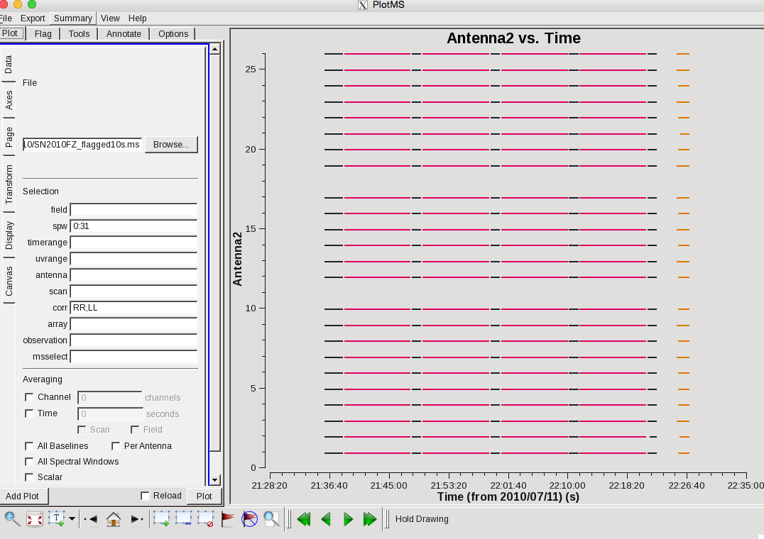
At this point it is useful to plot a "datastream" view of the dataset to show what antennas are present at what time. You can do this using
# In CASA
plotms(vis='SN2010FZ_flagged10s.ms',field='',correlation='RR,LL',
       timerange='',antenna='',spw='0:31',
       xaxis='time',yaxis='antenna2',
       plotrange=[-1,-1,0,26],coloraxis='field')
This shows the times where data is present on baselines TO a given Antenna2 (which means there is no line for ea01 which is antenna 0). You can pick up ea01 (and drop ea28) by setting yaxis='antenna1'. To the right we show this plot, having zoomed in on the last scan on 3C286. You see here that some antennas are present in this scan earlier than others (e.g. ea02 comes in one 10s integration later than ea04).
Calibration
Summarize the split flagged MS:
# In CASA
listobs('SN2010FZ_flagged10s.ms')
In the logger we see:
##########################################
##### Begin Task: listobs            #####

================================================================================
           MeasurementSet Name:  SN2010FZ_flagged10s.ms      MS Version 2
================================================================================
   Observer: Dr. Alicia M. Soderberg     Project: T.B.D.
Observation: EVLA
Data records: 1375038       Total integration time = 3042 seconds
   Observed from   11-Jul-2010/21:36:01.0   to   11-Jul-2010/22:26:43.0 (UTC)

   ObservationID = 0         ArrayID = 0
  Date        Timerange (UTC)          Scan  FldId FieldName           nRows   Int(s)   SpwIds      ScanIntent
  11-Jul-2010/21:36:01.0 - 21:38:20.5     7      0 J0925+0019          73710  9.93     [0, 1, 2, 3, 4, 5, 6, 7, 8, 9, 10, 11, 12, 13]CALIBRATE_PHASE#UNSPECIFIED
              21:38:44.0 - 21:39:51.0     9      1 SN2010FZ            39312  9.16     [0, 1, 2, 3, 4, 5, 6, 7, 8, 9, 10, 11, 12, 13]OBSERVE_TARGET#UNSPECIFIED
              21:40:01.0 - 21:41:20.5    10      1 SN2010FZ            44226  9.89     [0, 1, 2, 3, 4, 5, 6, 7, 8, 9, 10, 11, 12, 13]OBSERVE_TARGET#UNSPECIFIED
              21:41:30.0 - 21:42:50.0    11      1 SN2010FZ            44226  10       [0, 1, 2, 3, 4, 5, 6, 7, 8, 9, 10, 11, 12, 13]OBSERVE_TARGET#UNSPECIFIED
              21:43:00.0 - 21:44:20.0    12      1 SN2010FZ            44226  10       [0, 1, 2, 3, 4, 5, 6, 7, 8, 9, 10, 11, 12, 13]OBSERVE_TARGET#UNSPECIFIED
              21:44:30.0 - 21:45:50.0    13      1 SN2010FZ            44226  10       [0, 1, 2, 3, 4, 5, 6, 7, 8, 9, 10, 11, 12, 13]OBSERVE_TARGET#UNSPECIFIED
              21:46:00.0 - 21:47:19.5    14      1 SN2010FZ            44226  9.89     [0, 1, 2, 3, 4, 5, 6, 7, 8, 9, 10, 11, 12, 13]OBSERVE_TARGET#UNSPECIFIED
              21:47:29.0 - 21:47:49.0    15      1 SN2010FZ            14742  9.67     [0, 1, 2, 3, 4, 5, 6, 7, 8, 9, 10, 11, 12, 13]OBSERVE_TARGET#UNSPECIFIED
              21:48:12.0 - 21:49:18.5    16      0 J0925+0019          39312  9        [0, 1, 2, 3, 4, 5, 6, 7, 8, 9, 10, 11, 12, 13]CALIBRATE_PHASE#UNSPECIFIED
              21:49:42.0 - 21:50:49.0    17      1 SN2010FZ            39312  9.17     [0, 1, 2, 3, 4, 5, 6, 7, 8, 9, 10, 11, 12, 13]OBSERVE_TARGET#UNSPECIFIED
              21:50:59.0 - 21:52:19.0    18      1 SN2010FZ            44226  10       [0, 1, 2, 3, 4, 5, 6, 7, 8, 9, 10, 11, 12, 13]OBSERVE_TARGET#UNSPECIFIED
              21:52:29.0 - 21:53:48.5    19      1 SN2010FZ            44226  9.89     [0, 1, 2, 3, 4, 5, 6, 7, 8, 9, 10, 11, 12, 13]OBSERVE_TARGET#UNSPECIFIED
              21:53:58.0 - 21:55:18.0    20      1 SN2010FZ            44226  10       [0, 1, 2, 3, 4, 5, 6, 7, 8, 9, 10, 11, 12, 13]OBSERVE_TARGET#UNSPECIFIED
              21:55:28.0 - 21:56:48.0    21      1 SN2010FZ            44226  10       [0, 1, 2, 3, 4, 5, 6, 7, 8, 9, 10, 11, 12, 13]OBSERVE_TARGET#UNSPECIFIED
              21:56:58.0 - 21:58:18.0    22      1 SN2010FZ            44226  10       [0, 1, 2, 3, 4, 5, 6, 7, 8, 9, 10, 11, 12, 13]OBSERVE_TARGET#UNSPECIFIED
              21:58:28.0 - 21:58:47.5    23      1 SN2010FZ            14742  9.67     [0, 1, 2, 3, 4, 5, 6, 7, 8, 9, 10, 11, 12, 13]OBSERVE_TARGET#UNSPECIFIED
              21:59:10.5 - 22:00:17.0    24      0 J0925+0019          39312  8.99     [0, 1, 2, 3, 4, 5, 6, 7, 8, 9, 10, 11, 12, 13]CALIBRATE_PHASE#UNSPECIFIED
              22:00:39.5 - 22:01:47.0    25      1 SN2010FZ            39312  9.18     [0, 1, 2, 3, 4, 5, 6, 7, 8, 9, 10, 11, 12, 13]OBSERVE_TARGET#UNSPECIFIED
              22:01:57.0 - 22:03:17.0    26      1 SN2010FZ            44226  10       [0, 1, 2, 3, 4, 5, 6, 7, 8, 9, 10, 11, 12, 13]OBSERVE_TARGET#UNSPECIFIED
              22:03:27.0 - 22:04:47.0    27      1 SN2010FZ            44226  10       [0, 1, 2, 3, 4, 5, 6, 7, 8, 9, 10, 11, 12, 13]OBSERVE_TARGET#UNSPECIFIED
              22:04:57.0 - 22:06:16.5    28      1 SN2010FZ            44226  9.89     [0, 1, 2, 3, 4, 5, 6, 7, 8, 9, 10, 11, 12, 13]OBSERVE_TARGET#UNSPECIFIED
              22:06:26.0 - 22:07:46.0    29      1 SN2010FZ            44226  10       [0, 1, 2, 3, 4, 5, 6, 7, 8, 9, 10, 11, 12, 13]OBSERVE_TARGET#UNSPECIFIED
              22:07:56.0 - 22:09:16.0    30      1 SN2010FZ            44226  10       [0, 1, 2, 3, 4, 5, 6, 7, 8, 9, 10, 11, 12, 13]OBSERVE_TARGET#UNSPECIFIED
              22:09:26.0 - 22:09:45.5    31      1 SN2010FZ            14742  9.67     [0, 1, 2, 3, 4, 5, 6, 7, 8, 9, 10, 11, 12, 13]OBSERVE_TARGET#UNSPECIFIED
              22:10:08.0 - 22:11:15.5    32      0 J0925+0019          39312  9.13     [0, 1, 2, 3, 4, 5, 6, 7, 8, 9, 10, 11, 12, 13]CALIBRATE_PHASE#UNSPECIFIED
              22:11:38.0 - 22:12:45.5    33      1 SN2010FZ            39312  9.19     [0, 1, 2, 3, 4, 5, 6, 7, 8, 9, 10, 11, 12, 13]OBSERVE_TARGET#UNSPECIFIED
              22:12:55.0 - 22:14:15.0    34      1 SN2010FZ            44226  10       [0, 1, 2, 3, 4, 5, 6, 7, 8, 9, 10, 11, 12, 13]OBSERVE_TARGET#UNSPECIFIED
              22:14:25.0 - 22:15:45.0    35      1 SN2010FZ            44226  10       [0, 1, 2, 3, 4, 5, 6, 7, 8, 9, 10, 11, 12, 13]OBSERVE_TARGET#UNSPECIFIED
              22:15:55.0 - 22:17:15.0    36      1 SN2010FZ            44226  10       [0, 1, 2, 3, 4, 5, 6, 7, 8, 9, 10, 11, 12, 13]OBSERVE_TARGET#UNSPECIFIED
              22:17:25.0 - 22:18:44.5    37      1 SN2010FZ            44226  9.89     [0, 1, 2, 3, 4, 5, 6, 7, 8, 9, 10, 11, 12, 13]OBSERVE_TARGET#UNSPECIFIED
              22:18:54.0 - 22:20:14.0    38      1 SN2010FZ            44226  10       [0, 1, 2, 3, 4, 5, 6, 7, 8, 9, 10, 11, 12, 13]OBSERVE_TARGET#UNSPECIFIED
              22:20:24.0 - 22:20:43.5    39      1 SN2010FZ            14742  9.67     [0, 1, 2, 3, 4, 5, 6, 7, 8, 9, 10, 11, 12, 13]OBSERVE_TARGET#UNSPECIFIED
              22:21:06.0 - 22:22:13.5    40      0 J0925+0019          38584  9.15     [0, 1, 2, 3, 4, 5, 6, 7, 8, 9, 10, 11, 12, 13]CALIBRATE_PHASE#UNSPECIFIED
              22:25:13.0 - 22:25:13.0    42      2 3C286               924    2.88     [0, 1, 2, 3, 4, 5, 6, 7, 8, 9, 10, 11, 12, 13]CALIBRATE_BANDPASS#UNSPECIFIED,CALIBRATE_AMPLI#UNSPECIFIED
              22:25:23.0 - 22:26:43.0    43      2 3C286               43148  9.6      [0, 1, 2, 3, 4, 5, 6, 7, 8, 9, 10, 11, 12, 13]CALIBRATE_BANDPASS#UNSPECIFIED,CALIBRATE_AMPLI#UNSPECIFIED
           (nVis = Total number of time/baseline visibilities per scan)
Fields: 3
  ID   Code Name                RA              Decl          Epoch   SrcId nVis
  0    D    J0925+0019          09:25:07.81503 +00.19.13.9334 J2000   0     230230
  1    NONE SN2010FZ            09:42:04.77000 +00.19.51.0000 J2000   1     1100736
  2    K    3C286               13:31:08.28798 +30.30.32.9589 J2000   2     44072
   (nVis = Total number of time/baseline visibilities per field)
Spectral Windows:  (14 unique spectral windows and 1 unique polarization setups)
  SpwID  #Chans Frame Ch1(MHz)    ChanWid(kHz)  TotBW(kHz)  Corrs
  0          64 TOPO  4488        2000          128000      RR  RL  LR  LL
  1          64 TOPO  4616        2000          128000      RR  RL  LR  LL
  2          64 TOPO  4744        2000          128000      RR  RL  LR  LL
  3          64 TOPO  4872        2000          128000      RR  RL  LR  LL
  4          64 TOPO  5000        2000          128000      RR  RL  LR  LL
  5          64 TOPO  5128        2000          128000      RR  RL  LR  LL
  6          64 TOPO  5256        2000          128000      RR  RL  LR  LL
  7          64 TOPO  5384        2000          128000      RR  RL  LR  LL
  8          64 TOPO  6744        2000          128000      RR  RL  LR  LL
  9          64 TOPO  6872        2000          128000      RR  RL  LR  LL
  10         64 TOPO  7000        2000          128000      RR  RL  LR  LL
  11         64 TOPO  7128        2000          128000      RR  RL  LR  LL
  12         64 TOPO  7256        2000          128000      RR  RL  LR  LL
  13         64 TOPO  7384        2000          128000      RR  RL  LR  LL
<snip>
Note that the spectral windows are re-numbered to 0 through 13.
Setting the flux density scale
It is now time to begin calibrating the data. The general data reduction strategy is to derive a series of scaling factors or corrections from the calibrators, which are then collectively applied to the science data. For much more discussion of the philosophy, strategy, and implementation of calibration of synthesis data within CASA, see Synthesis Calibration in the CASA Cookbook and User Reference Manual .
Before calibrating, we insert a model for flux calibration source 3C286 into the MS. In order to do this, we first have to locate the model image on our system with setjy, which we will also use to set the flux density scale. The setjy task (in release 3.3.0 and later) has an option to list possible model images it knows about:
# In CASA
setjy(vis='SN2010FZ_flagged10s.ms', listmodels=True)
which sends output to your terminal (but not the logger). For example, on an NRAO workstation:
No candidate modimages matching '*.im* *.mod*' found in .

Candidate modimages (*) in /usr/lib64/casapy/release/4.2.0/data/nrao/VLA/CalModels:
3C138_A.im  3C138_S.im  3C147_K.im  3C147_X.im  3C286_Q.im  3C48_C.im  3C48_U.im
3C138_C.im  3C138_U.im  3C147_L.im  3C286_A.im  3C286_S.im  3C48_K.im  3C48_X.im
3C138_K.im  3C138_X.im  3C147_Q.im  3C286_C.im  3C286_U.im  3C48_L.im  README
3C138_L.im  3C147_A.im  3C147_S.im  3C286_K.im  3C286_X.im  3C48_Q.im
3C138_Q.im  3C147_C.im  3C147_U.im  3C286_L.im  3C48_A.im   3C48_S.im
The relevant image for our purposes is 3C286_C.im, in the directory /usr/lib64/casapy/release/data/nrao/VLA/CalModels. Your system may show a different location (for example /home/casa/data/nrao/VLA/CalModels/, or /Applications/CASA.app/Contents/data/nrao/VLA/CalModels on a Mac). Since it knows about this image, we only have to give the image name and not the entire path. Otherwise, you will need to give it the entire path. We now run the task using this model:
# In CASA
mysetjy = setjy(vis='SN2010FZ_flagged10s.ms', field='2', scalebychan=True, model='3C286_C.im', usescratch=False)
- scalebychan=True: will fill the model with per-channel values; otherwise, setjy would use a single value per spectral window.
- usescratch=False: put the model in the header instead of creating scratch columns in the MS. This will take up considerably less disk space.
We have not specified a Flux Density Scale Standard and are thus using the default (standard='Perley-Butler 2010') as that was current when these observations were taken. In particular, there is a more recent "Perley-Butler 2013" scale that most users will want to use! See help setjy for more details.
Inspecting the logger report shows that 3C286 is about 7.7 Jy at lower end of the band to 5.7 Jy at the upper end.
Note: With release 4.2 setjy now returns a dictionary to Python, which we have captured in a variable. This can be used in scripts.
Deriving pre-determined calibrations: antenna position corrections, gain-elevation curves, and requantizer gains
Some calibration products are carried along throughout the calibration process and used as priors for subsequent calibration steps. These include the antenna position corrections, gain-elevation curves, and requantizer gains.
We use gencal to determine any antenna-position corrections that need to be applied to the data. This is based on a database of corrections with the time they were determined and when they were applied by the observing system, compared to the times in your observations.
# In CASA
gencal('SN2010FZ_flagged10s.ms',caltable='calSN2010FZ.antpos',caltype='antpos',antenna='')
You should see in the logger:
Determine antenna position offests from the baseline correction database
offsets for antenna ea01 :  0.00000   0.00300   0.00000
offsets for antenna ea02 : -0.00080   0.00000   0.00000
offsets for antenna ea03 : -0.00280   0.00000   0.00000
offsets for antenna ea05 :  0.00000   0.00280   0.00000
offsets for antenna ea06 :  0.00220   0.00100   0.00590
offsets for antenna ea10 :  0.00080   0.00300  -0.00140
offsets for antenna ea11 :  0.00090   0.00000   0.00000
offsets for antenna ea12 : -0.00280   0.00000   0.00000
offsets for antenna ea13 :  0.00000  -0.00080   0.00000
offsets for antenna ea17 : -0.00120   0.00000   0.00000
offsets for antenna ea18 :  0.00040  -0.00080   0.00040
offsets for antenna ea22 : -0.00370  -0.00130   0.00000
offsets for antenna ea23 : -0.00140   0.00000   0.00000
offsets for antenna ea24 : -0.00150   0.00000   0.00000
offsets for antenna ea26 : -0.00190   0.00000   0.00210
offsets for antenna ea27 :  0.00000   0.00190  -0.00160
Note that there are significant position corrections for a number of the antennas.
In CASA 4.1 and later, we now have the option to use gencal to create a calibration table containing the gain curves for the antennas. Although you can still use the gaincurve=True option in each task, we will make use of this new feature (note that the gaincurve=True will be phased out in future CASA releases):
# In CASA
gencal('SN2010FZ_flagged10s.ms',caltable='calSN2010FZ.gaincurve',caltype='gc')
Finally, we will use gencal to create a calibration table containing corrections for the requantizer gains. Although this is only necessary for 3-bit data (and our SN2010FZ is 8-bit), we include it here for completeness. It will not affect the calibration for our 8-bit data, but if one is following this CASA Guide as a template for 3-bit data, this step is needed to account for the small gain changes (~5-10%) that result from resetting the quantizer gains as the correlator changes to a new 3-bit configuration.
# In CASA
gencal('SN2010FZ_flagged10s.ms',caltable='calSN2010FZ.requantizer',caltype='rq')
Since we're running gencal on 3-bit data, it logs that it found "0 TIME/SPW switched power samples."
The caltables we have generated -- calSN2010FZ.antpos, calSN2010FZ.gaincurve, and calSN2010FZ.requantizer -- will need to be pre-applied in subsequent calibration steps.
Calibrating delays and bandpass
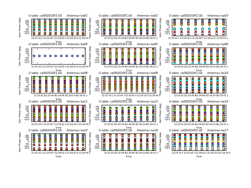
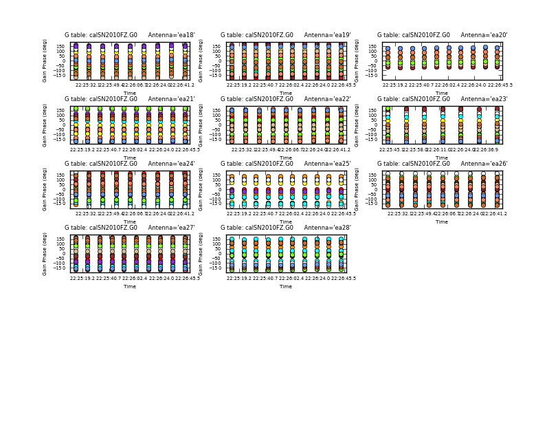
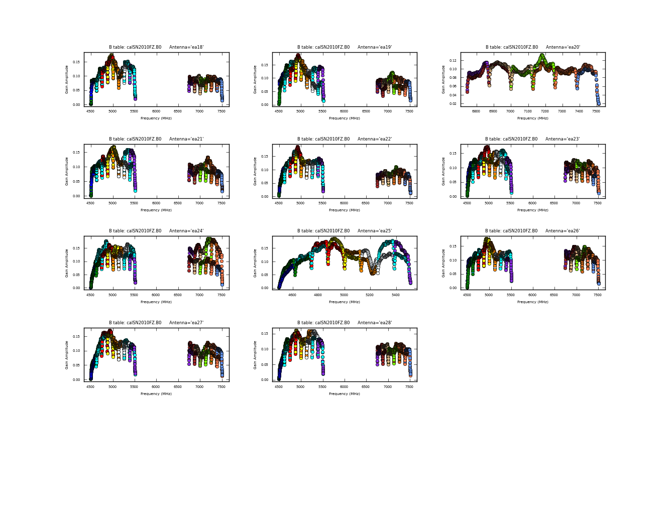
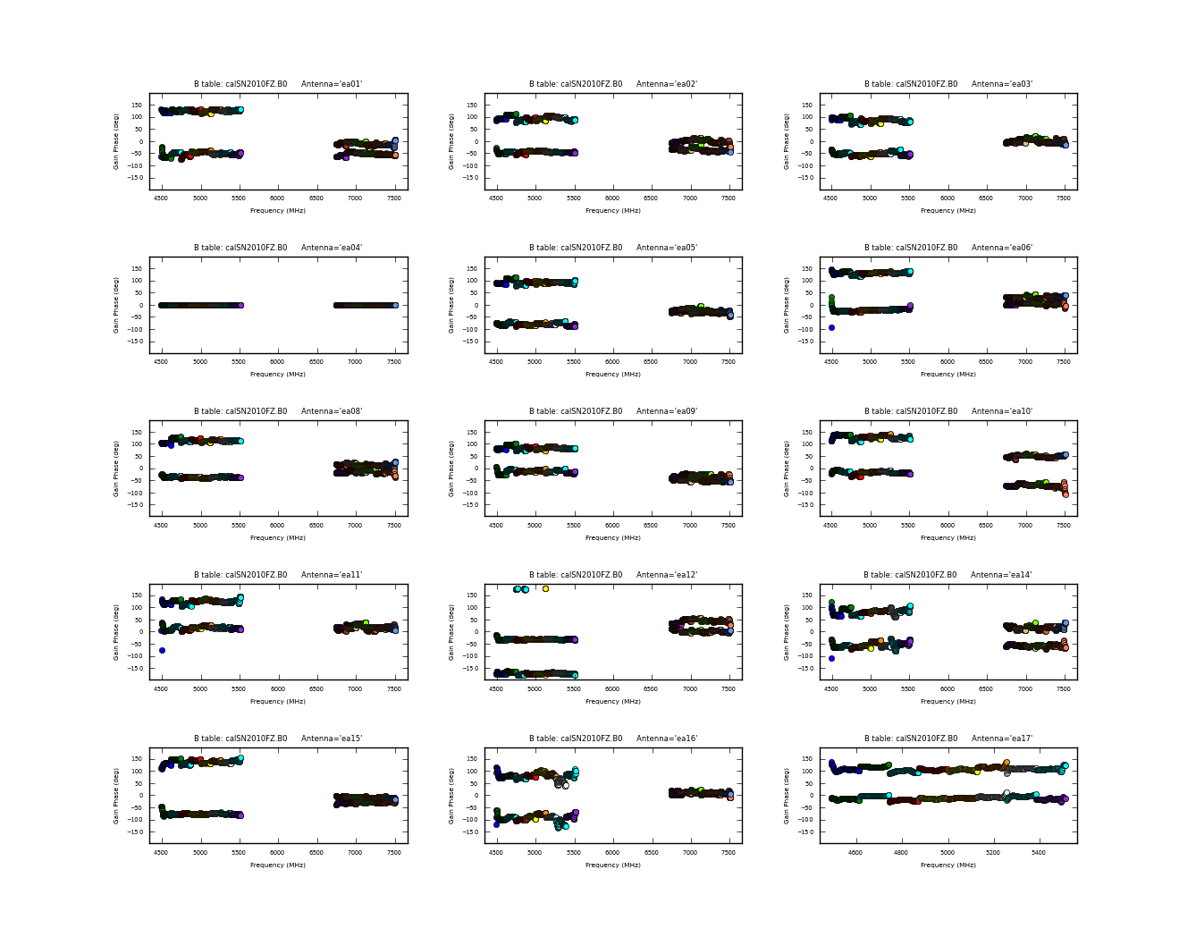
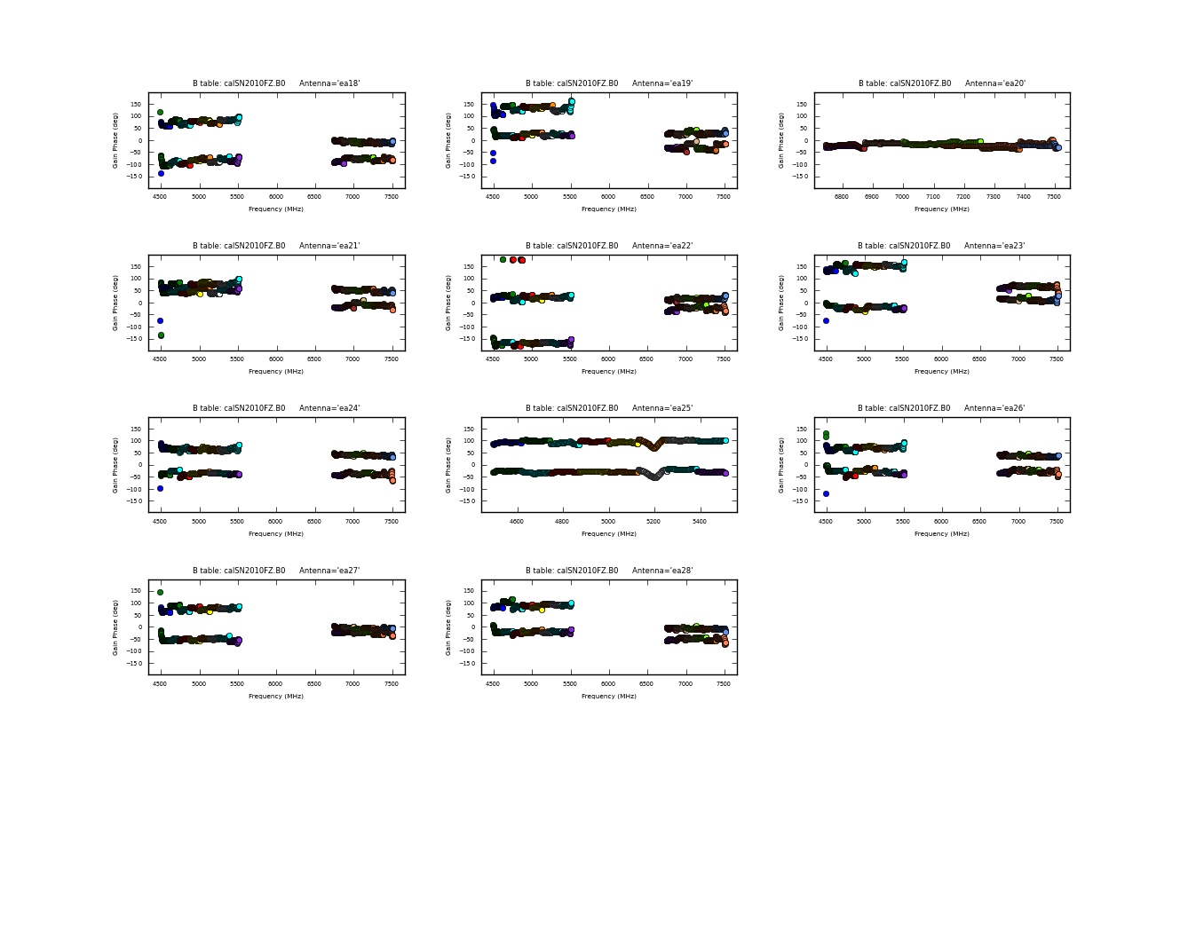
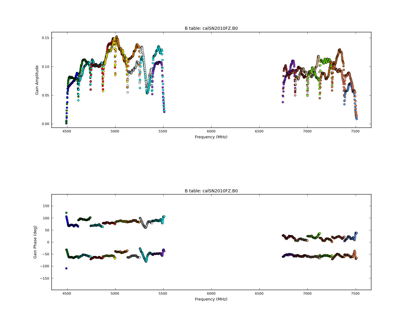
First, we do a phase-only calibration solution on a narrow range of channels in each spw on the bandpass/flux calibrator 3c286 to flatten them before solving for the bandpass. Note where we saw RFI in the higher spw and avoid those channels. The range 23~28 should work. Pick a refant near center - ea04 is a reasonable bet (see above):
# In CASA
gaincal(vis='SN2010FZ_flagged10s.ms',caltable='calSN2010FZ.G0',field='2',spw='0~13:23~28', \
        gaintable=['calSN2010FZ.antpos','calSN2010FZ.gaincurve'],\
        gaintype='G',refant='ea04',calmode='p',solint='int',minsnr=3)
- refant='ea04' : try to use ea04 as the reference antenna
- solint='int' : do a per-integration solve (every 10 seconds, since we've time-averaged the data)
- minsnr=3 : apply a minimum signal-to-noise cutoff. Solutions with less than this value will be flagged
- gaintable=['calSN2010FZ.antpos','calSN2010FZ.gaincurve'] : pre-apply the antpos and gaincurve caltables
Plot the phase solutions (using full phase range, -180 to 180, instead of autorange):
# In CASA
plotcal(caltable='calSN2010FZ.G0',xaxis='time',yaxis='phase',iteration='antenna', \
        plotrange=[-1,-1,-180,180])
Step through the antenna-based solutions. They look good (and fairly flat over the scans).
NOTE: When you are done plotting and want to use the caltable in another task, use the Quit button on the GUI to dismiss the plotter and free up the lock on the caltable. You should see a message in your terminal window saying "Resetting plotcal" which means you are good to go!
If you want to make single-page multipanel plots (like those shown to the right), particularly for a hardcopy (where it only shows the first page), you can do:
# In CASA
plotcal(caltable='calSN2010FZ.G0',xaxis='time',yaxis='phase', \
        antenna='0~10,12~15',subplot=531,iteration='antenna', \
        plotrange=[-1,-1,-180,180],showgui=False,fontsize=6.0, \
        figfile='plotSN2010FZ_plotcal_G0p1.png')
plotcal(caltable='calSN2010FZ.G0',xaxis='time',yaxis='phase', \
        antenna='16~26',subplot=531,iteration='antenna', \
        plotrange=[-1,-1,-180,180],showgui=False,fontsize=6.0, \
        figfile='plotSN2010FZ_plotcal_G0p2.png')
We can now solve for the residual antenna-based delays that we saw in phase vs. frequency. This uses the new gaintype='K' option in gaincal. Note that this currently does not do a "global fringe-fitting" solution for delays, but instead does a baseline-based delay solution to all baselines to the refant, treating these as antenna-based delays. In most cases with high-enough S/N to get baseline-based delay solutions this will suffice. We avoid the beginning of spw 0 due to the extreme roll-off (with loss of S/N) at the starting edge.
# In CASA
gaincal(vis='SN2010FZ_flagged10s.ms',caltable='calSN2010FZ.K0',\
        gaintable=['calSN2010FZ.antpos','calSN2010FZ.gaincurve','calSN2010FZ.G0'],\
        field='2',spw='0:8~59,1~13:4~59',gaintype='K', \
        refant='ea04',combine='scan',solint='inf',minsnr=3)
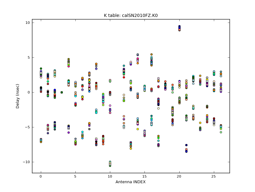
We pre-apply our initial phase table, and produce a new K-type caltable for input to bandpass calibration. We can plot the delays, in nanoseconds, as a function of antenna index (you will get one for each subband and polarization):
# In CASA
plotcal(caltable='calSN2010FZ.K0', xaxis='antenna', yaxis='delay')
The delays range from around -6 to 6 nanoseconds.
Now solve for the bandpass using the previous tables:
# In CASA
bandpass(vis='SN2010FZ_flagged10s.ms',caltable='calSN2010FZ.B0', \
         gaintable=['calSN2010FZ.antpos','calSN2010FZ.gaincurve', \
                    'calSN2010FZ.G0','calSN2010FZ.K0'], \
         field='2',refant='ea04',solnorm=False, \
         bandtype='B', combine='scan', solint='inf')
WARNING: You must set solnorm=False here or later on you will find some offsets between spw due to how amplitude scaling adjusts weights internally during solving.
You will see in the terminal some reports of solutions failing below our default S/N>3 cutoff:
32 of 50 solutions flagged due to SNR < 3 in spw=0 (chan=1) at 2010/07/11/22:26:05.4
44 of 50 solutions flagged due to SNR < 3 in spw=0 (chan=0) at 2010/07/11/22:26:05.4
These are in the first two edge channels of the first spw where the response is low, and not unexpected. In the logger you will also see reports of reference antennas jumping in those channels, which can be be safely ignored (we will drop those channels later anyway).
This is the first amplitude-scaling calibration that we do, so it is important to have used the calSN2010FZ.gaincurve caltable (or set gaincurve=True). If we were at higher frequency we would also have made an opacity caltable (or set opacity).
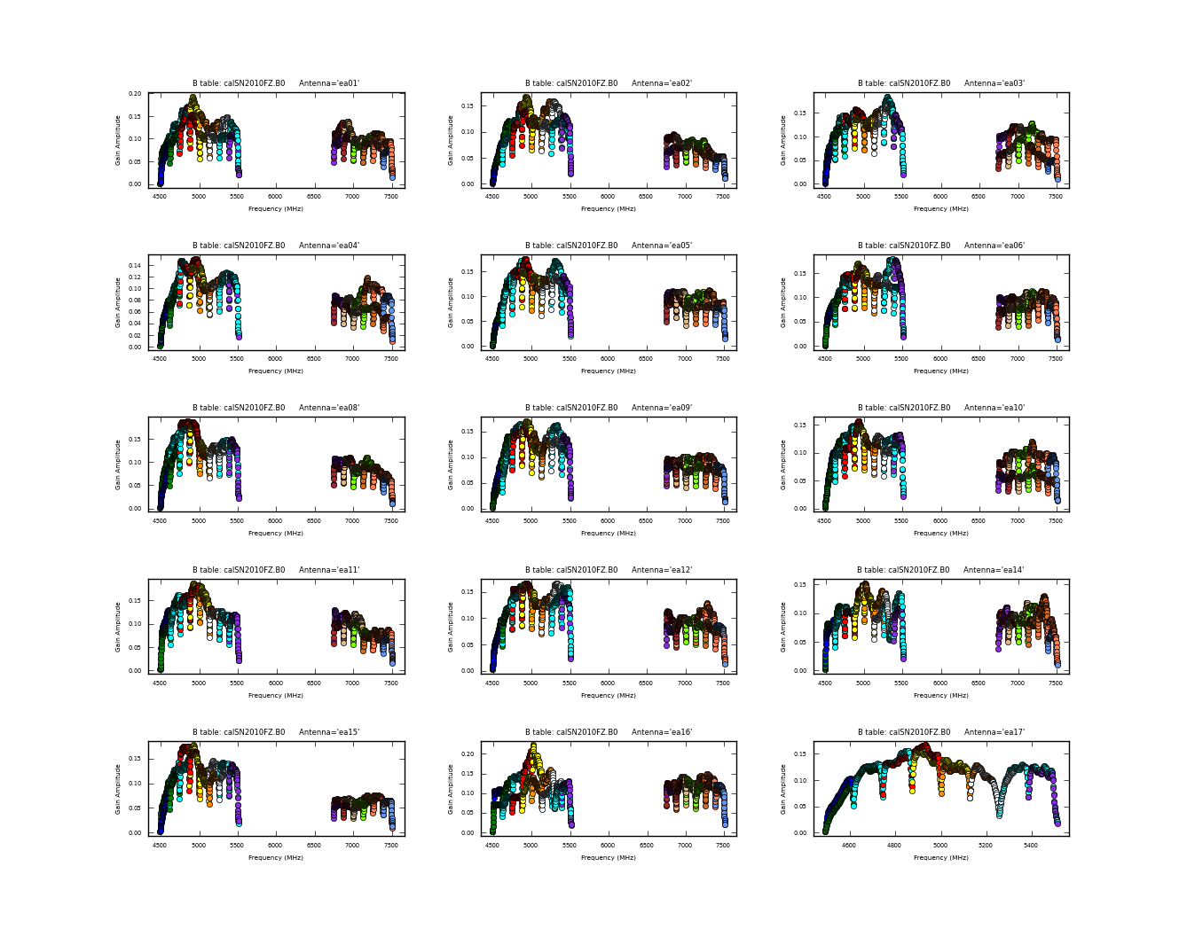
Now plot this, in amplitude then phase:
# In CASA
plotcal(caltable='calSN2010FZ.B0',xaxis='freq',yaxis='amp',iteration='antenna')
#
plotcal(caltable='calSN2010FZ.B0',xaxis='freq',yaxis='phase',iteration='antenna', \
        plotrange=[-1,-1,-180,180])
or to plot them all together
# In CASA
plotcal(caltable='calSN2010FZ.B0',xaxis='freq',yaxis='amp',
        antenna='0~10,12~15',subplot=531,iteration='antenna',
        fontsize=6.0, figfile='plotSN2010FZ_plotcal_B0a1_4.2.png')
plotcal(caltable='calSN2010FZ.B0',xaxis='freq',yaxis='amp',
        antenna='16~26',subplot=531,iteration='antenna',
        fontsize=6.0, figfile='plotSN2010FZ_plotcal_B0a2_4.2.png')
#
plotcal(caltable='calSN2010FZ.B0',xaxis='freq',yaxis='phase',
        antenna='0~10,12~15',subplot=531,iteration='antenna',
        plotrange=[-1,-1,-180,180],fontsize=6.0,
        figfile='plotSN2010FZ_plotcal_B0p1_4.2.png')
plotcal(caltable='calSN2010FZ.B0',xaxis='freq',yaxis='phase',
        antenna='16~26',subplot=531,iteration='antenna',
        plotrange=[-1,-1,-180,180],fontsize=6.0,
        figfile='plotSN2010FZ_plotcal_B0p2_4.2.png')
(this can take a long time to plot).
In the bandpass phase you no longer see the residual antenna delays (just residual spw phase offsets from the delay solution registration) but there are some band edge effects. Note that some antennas have a little strange bandpasses at upper end of lower baseband in spw 5,6,7 (e.g. ea14,ea16,ea17,ea25). To plot amp and phase for a single antenna versus frequency (see plots at right):
# In CASA
plotcal(caltable='calSN2010FZ.B0',xaxis='freq',yaxis='amp', \
        antenna='ea14',subplot=211)
plotcal(caltable='calSN2010FZ.B0',xaxis='freq',yaxis='phase', \
        antenna='ea14',subplot=212,plotrange=[-1,-1,-180,180])
Because our flux density calibrator 3C286 is bright enough, we were able to use this as the bandpass calibrator. Since setjy put the correct spectrum for 3C286 into the MODEL_DATA column, our bandpass will reflect the true bandpass of the instrument. However, if for your observation you were unable to use a source of known spectrum as the bandpass calibrator, then you would need to use the output of fluxscale later on to bootstrap a setjy on your bandpass source using the derived spectral index information.
Final phase and amplitude calibration
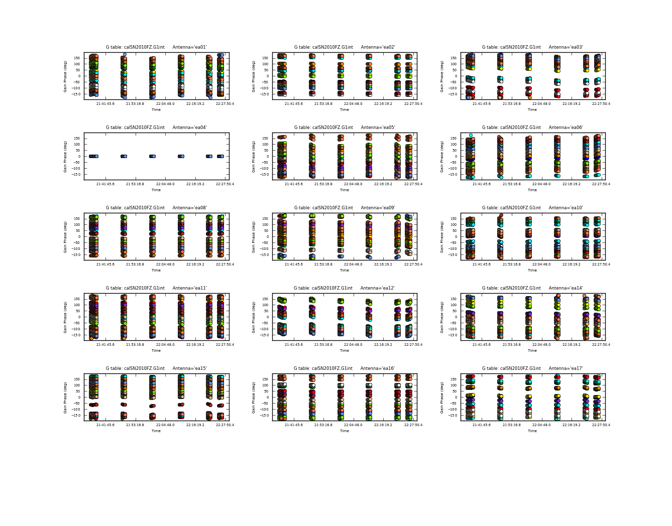
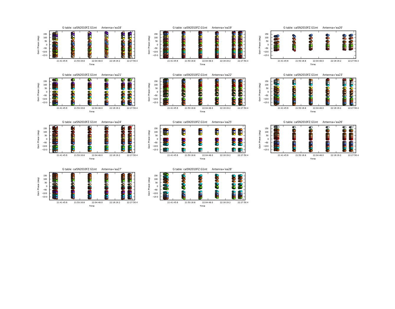

Now calibrate phases using the full bandwidth. First both our calibrators, one at a time - we could do them together, but in general you might need to do different solution intervals for each, so we keep the runs separate to illustrate how to do separate solutions and append them. We exclude RFI channels here, and obtain one solution per integration (these are bright enough):
# In CASA
gaincal(vis='SN2010FZ_flagged10s.ms',caltable='calSN2010FZ.G1int', \
        gaintable=['calSN2010FZ.antpos','calSN2010FZ.gaincurve',
                   'calSN2010FZ.K0','calSN2010FZ.B0'], \
        field='2',refant='ea04',solnorm=F, \
        spw='0:10~59,1~7:4~59,8:4~13;18~59,9~11:4~59,12:4~13;18~29;31~33;46~51;53~59,13:4~8;15~36;42~59', \
        solint='int',gaintype='G',calmode='p')
#
gaincal(vis='SN2010FZ_flagged10s.ms',caltable='calSN2010FZ.G1int', \
        gaintable=['calSN2010FZ.antpos','calSN2010FZ.gaincurve',
                   'calSN2010FZ.K0','calSN2010FZ.B0'], \
        field='0',refant='ea04',solnorm=F, \
        spw='0:10~59,1~7:4~59,8:4~13;18~59,9~11:4~59,12:4~13;18~29;31~33;46~51;53~59,13:4~8;15~36;42~59', \
        solint='int',gaintype='G',calmode='p',append=True)
These will get applied when solving for amplitudes, and when calibrating the calibrators themselves.
The phases look reasonably connected:
# In CASA
plotcal(caltable='calSN2010FZ.G1int',xaxis='time',yaxis='phase',iteration='antenna', \
        plotrange=[-1,-1,-180,180])
To apply phase calibration to the target, we make a second table with one solution on our gain calibrator per scan:
# In CASA
gaincal(vis='SN2010FZ_flagged10s.ms',caltable='calSN2010FZ.G1inf',
        gaintable=['calSN2010FZ.antpos','calSN2010FZ.gaincurve',
                   'calSN2010FZ.K0','calSN2010FZ.B0'], \
        field='0',refant='ea04',solnorm=F, \
        spw='0:10~59,1~7:4~59,8:4~13;18~59,9~11:4~59,12:4~13;18~29;31~33;46~51;53~59,13:4~8;15~36;42~59', \
        solint='inf',gaintype='G',calmode='p')
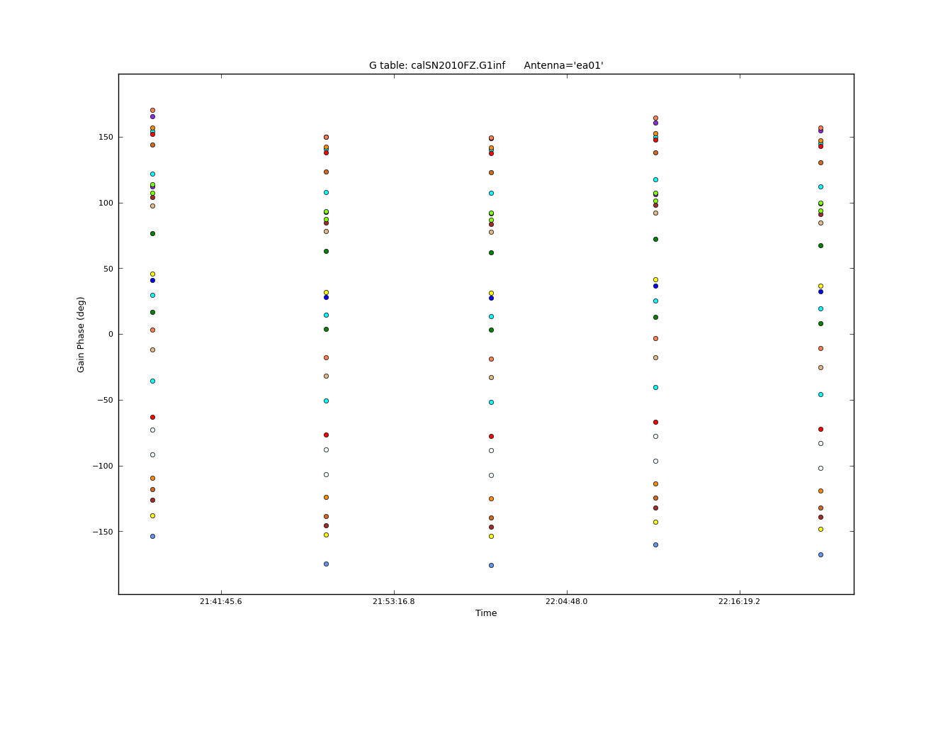
These scan phases will get interpolated by applycal onto our target. These look good also:
# In CASA
plotcal(caltable='calSN2010FZ.G1inf',xaxis='time',yaxis='phase',iteration='antenna', \
        plotrange=[-1,-1,-180,180])
Now solve for amplitudes on a per scan interval, after applying the per-integration phases. Do these separately using gainfield so phases don't get transferred across fields. For field 2 (3C286) we use combine='scan' as there are two scans on this source, with the first one having much less data (and will thus give a noisy solution on its own). Note that gaincal uses linear interpolation of the previously determined phases by default, so set this to "nearest" if you want to override this.
# In CASA
gaincal(vis='SN2010FZ_flagged10s.ms', caltable='calSN2010FZ.G2', \
        gaintable=['calSN2010FZ.antpos','calSN2010FZ.gaincurve',
                   'calSN2010FZ.K0','calSN2010FZ.B0','calSN2010FZ.G1int'], \
        gainfield=['','','2','2','2'], \
        interp=['','','nearest','nearest','nearest'], \
        field='2',refant='ea04',solnorm=F,
        spw='0:10~59,1~7:4~59,8:4~13;18~59,9~11:4~59,12:4~13;18~29;31~33;46~51;53~59,13:4~8;15~36;42~59', \
        solint='inf',combine='scan',gaintype='G',calmode='a')
#
gaincal(vis='SN2010FZ_flagged10s.ms', caltable='calSN2010FZ.G2', \
        gaintable=['calSN2010FZ.antpos','calSN2010FZ.gaincurve',
                   'calSN2010FZ.K0','calSN2010FZ.B0','calSN2010FZ.G1int'],\
        gainfield=['','','2','2','0'], \
        interp=['','','nearest','nearest','nearest'], \
        field='0',refant='ea04',solnorm=F, \
        spw='0:10~59,1~7:4~59,8:4~13;18~59,9~11:4~59,12:4~13;18~29;31~33;46~51;53~59,13:4~8;15~36;42~59', \
        solint='inf',gaintype='G',calmode='a',append=True)
This is the table we will apply to the data.
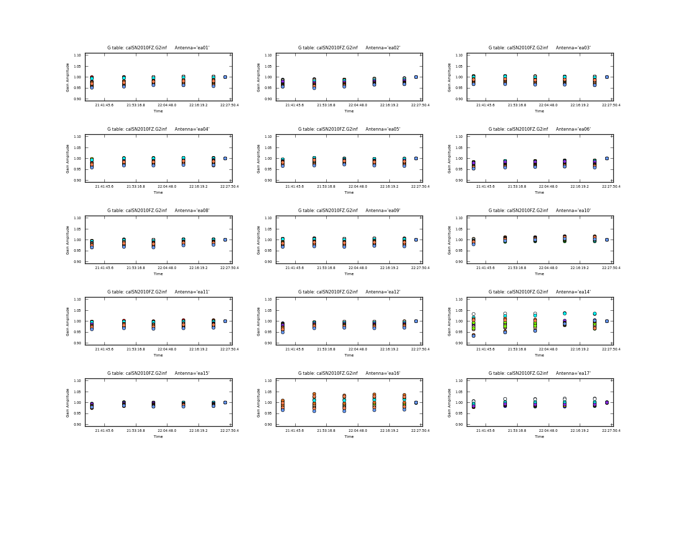
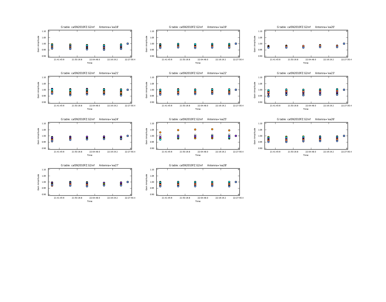
We do a second version of the amplitude calibration, this time using combine='scan' on field 0. This is to use for input to fluxscale in the next step.
# In CASA
gaincal(vis='SN2010FZ_flagged10s.ms', caltable='calSN2010FZ.G3', \
        gaintable=['calSN2010FZ.antpos','calSN2010FZ.gaincurve',
                   'calSN2010FZ.K0','calSN2010FZ.B0','calSN2010FZ.G1int'], \
        gainfield=['','','2','2','2'], \
        interp=['','','nearest','nearest','nearest'], \
        field='2',refant='ea04',solnorm=F,
        spw='0:10~59,1~7:4~59,8:4~13;18~59,9~11:4~59,12:4~13;18~29;31~33;46~51;53~59,13:4~8;15~36;42~59', \
        solint='inf',combine='scan',gaintype='G',calmode='a')
#
gaincal(vis='SN2010FZ_flagged10s.ms', caltable='calSN2010FZ.G3', \
        gaintable=['calSN2010FZ.antpos','calSN2010FZ.gaincurve',
                   'calSN2010FZ.K0','calSN2010FZ.B0','calSN2010FZ.G1int'],\
        gainfield=['','','2','2','0'], \
        interp=['','','nearest','nearest','nearest'], \
        field='0',refant='ea04',solnorm=F, \
        spw='0:10~59,1~7:4~59,8:4~13;18~59,9~11:4~59,12:4~13;18~29;31~33;46~51;53~59,13:4~8;15~36;42~59', \
        solint='inf',combine='scan',gaintype='G',calmode='a',append=True)
Since the flux on the gain calibrator is not scaled to its correct flux (but to 1.0 Jy by default), use fluxscale to transfer the amplitude gains from 3c286:
# In CASA
myflux = fluxscale(vis='SN2010FZ_flagged10s.ms',caltable='calSN2010FZ.G3', \
                   fluxtable='calSN2010FZ.F3inc',reference='2',transfer='0',
                   incremental=True)
where we have captured the returned dictionary in the Python variable myflux. We have use the incremental=True option (new to CASA 4.0) to make this table contain only the scale factors per-antenna per-spw per-field needed to scale the data (rather than rescaling the input table). Thus it can be applied in addition to our G2 table even though it was derived from the G3 table.
The logger output gives:
Found reference field(s): 3C286
Found transfer field(s):  J0925+0019
Flux density for J0925+0019 in SpW=0 (freq=4.488e+09 Hz) is: 0.977483 +/- 0.00278572 (SNR = 350.891, N = 50)
Flux density for J0925+0019 in SpW=1 (freq=4.616e+09 Hz) is: 0.975972 +/- 0.00253876 (SNR = 384.429, N = 50)
Flux density for J0925+0019 in SpW=2 (freq=4.744e+09 Hz) is: 0.978538 +/- 0.00242824 (SNR = 402.982, N = 50)
Flux density for J0925+0019 in SpW=3 (freq=4.872e+09 Hz) is: 0.979278 +/- 0.00244155 (SNR = 401.088, N = 50)
Flux density for J0925+0019 in SpW=4 (freq=5e+09 Hz) is: 0.981804 +/- 0.00219239 (SNR = 447.823, N = 50)
Flux density for J0925+0019 in SpW=5 (freq=5.128e+09 Hz) is: 0.981478 +/- 0.00314805 (SNR = 311.773, N = 50)
Flux density for J0925+0019 in SpW=6 (freq=5.256e+09 Hz) is: 0.985493 +/- 0.00343534 (SNR = 286.869, N = 50)
Flux density for J0925+0019 in SpW=7 (freq=5.384e+09 Hz) is: 0.978491 +/- 0.00201807 (SNR = 484.865, N = 50)
Flux density for J0925+0019 in SpW=8 (freq=6.744e+09 Hz) is: 0.959005 +/- 0.00260159 (SNR = 368.623, N = 48)
Flux density for J0925+0019 in SpW=9 (freq=6.872e+09 Hz) is: 0.955123 +/- 0.00262785 (SNR = 363.462, N = 48)
Flux density for J0925+0019 in SpW=10 (freq=7e+09 Hz) is: 0.954202 +/- 0.00281227 (SNR = 339.3, N = 48)
Flux density for J0925+0019 in SpW=11 (freq=7.128e+09 Hz) is: 0.950797 +/- 0.00354085 (SNR = 268.522, N = 48)
Flux density for J0925+0019 in SpW=12 (freq=7.256e+09 Hz) is: 0.94732 +/- 0.00391511 (SNR = 241.965, N = 48)
Flux density for J0925+0019 in SpW=13 (freq=7.384e+09 Hz) is: 0.939356 +/- 0.00383532 (SNR = 244.922, N = 48)
Fitted spectrum for J0925+0019 with fitorder=1: Flux density = 0.968048 +/- 0.00159415 (freq=5.74863 GHz)
    spidx=-0.0721976 +/- 0.00943577
...
You may see slightly different numbers on your machine (and will see more extensive output). Note that "N" here is the number of antennas x the number of polarizations used for the calculations; in this case, there are 24 unflagged antennas and 2 polarizations. As of CASA 4.0, fluxscale now returns a fitted spectral index (and possibly curvature, e.g. if fitorder>1), which can be input to setjy if you want to use these derived fluxes for a model.
As it so happens, the derived flux for J0925+0019 is about 1 Jy (you can plot up the raw amplitudes for fields 0,2 and convince yourself this is indeed true and not a bug). The spectrum rises a bit to peak in spw 6 then falls again. We will not use the fitted spectrum (setjy does not yet take fitorder>1) but will apply a incremental table in subsequent processing.
Applying the Calibration and Final Editing
Next we actually apply all our accumulated calibration tables. We apply these to the calibration fields individually using the appropriate gainfields and interpolation for each:
- For 3C286 (field 2) we did short-timescale phase solutions and a single scan amplitude, so use "linear" and "nearest" interpolation respectively.
- For the nearby gain calibrator (field 0) we did only scan-based phase and amplitude solutions so we use "nearest" interpolation
- For the target source we use field 0 to calibrate field 1, so use "linear" interpolation. This takes a few minutes.

# In CASA
applycal(vis='SN2010FZ_flagged10s.ms',field='2', \
         gaintable=['calSN2010FZ.antpos','calSN2010FZ.gaincurve','calSN2010FZ.K0',
                    'calSN2010FZ.B0','calSN2010FZ.G1int','calSN2010FZ.G2'], \
         gainfield=['','','','','2','2'],
         interp=['','','nearest','nearest','nearest','nearest'], \
         parang=False,calwt=False)
#
applycal(vis='SN2010FZ_flagged10s.ms',field='0', \
         gaintable=['calSN2010FZ.antpos','calSN2010FZ.gaincurve','calSN2010FZ.K0',
                    'calSN2010FZ.B0','calSN2010FZ.G1int','calSN2010FZ.G2',
                    'calSN2010FZ.F3inc'], \
         gainfield=['','','','','0','0','0'],
         interp=['','','nearest','nearest','nearest','nearest',''], \
         parang=False,calwt=False)
#
applycal(vis='SN2010FZ_flagged10s.ms',field='1', \
         gaintable=['calSN2010FZ.antpos','calSN2010FZ.gaincurve','calSN2010FZ.K0',
                    'calSN2010FZ.B0','calSN2010FZ.G1inf','calSN2010FZ.G2',
                    'calSN2010FZ.F3inc'], \
         gainfield=['','','','','0','0','0'],
         interp=['','','nearest','nearest','linear','linear',''], \
         parang=False,calwt=False)
Because we used usesratch=False in setjy, the CORRECTED_DATA scratch column will be created the first time you run applycal. This will store the calibrated data.
We can examine the corrected data on 3c286 using our RFI mask from above and avoiding band edges
# In CASA
plotms(vis='SN2010FZ_flagged10s.ms',field='2', \
       spw='0:10~59,1~7:4~59,8:4~13;18~59,9~11:4~59,12:4~13;18~29;31~33;46~51;53~59,13:4~8;15~36;42~59', \
       correlation='RR,LL',xaxis='frequency',yaxis='amp',ydatacolumn='corrected')
See figure above right. There is clearly discrepant data visible spw 5 and 6, in particular for baseline ea17&ea25 (use the Mark Regions ![]() tool on some of it and then use the Locate
tool on some of it and then use the Locate ![]() tool), which gives a really strange response. You can plot just this baseline to be sure:
tool), which gives a really strange response. You can plot just this baseline to be sure:
# In CASA
plotms(vis='SN2010FZ_flagged10s.ms',field='2', \
       spw='0:10~59,1~7:4~59,8:4~13;18~59,9~11:4~59,12:4~13;18~29;31~33;46~51;53~59,13:4~8;15~36;42~59', \
       antenna='ea17&ea25', \
       correlation='RR,LL',xaxis='frequency',yaxis='amp',ydatacolumn='corrected')
You can exclude this through antenna negation:
# In CASA
plotms(vis='SN2010FZ_flagged10s.ms',field='2', \
       spw='0:10~59,1~7:4~59,8:4~13;18~59,9~11:4~59,12:4~13;18~29;31~33;46~51;53~59,13:4~8;15~36;42~59', \
       antenna='!ea17&ea25', \
       correlation='RR,LL',xaxis='frequency',yaxis='amp',ydatacolumn='corrected')
Then use Locate ![]() for the other bad points, which seem to indicate spw 5,6,7 for ea14,ea16,ea17,ea25.
Exclude these and replot:
for the other bad points, which seem to indicate spw 5,6,7 for ea14,ea16,ea17,ea25.
Exclude these and replot:
# In CASA
plotms(vis='SN2010FZ_flagged10s.ms',field='2', \
       spw='0:10~59,1~7:4~59,8:4~13;18~59,9~11:4~59,12:4~13;18~29;31~33;46~51;53~59,13:4~8;15~36;42~59', \
       antenna='!ea14;!ea16;!ea17;!ea25', \
       correlation='RR,LL',xaxis='frequency',yaxis='amp',ydatacolumn='corrected')

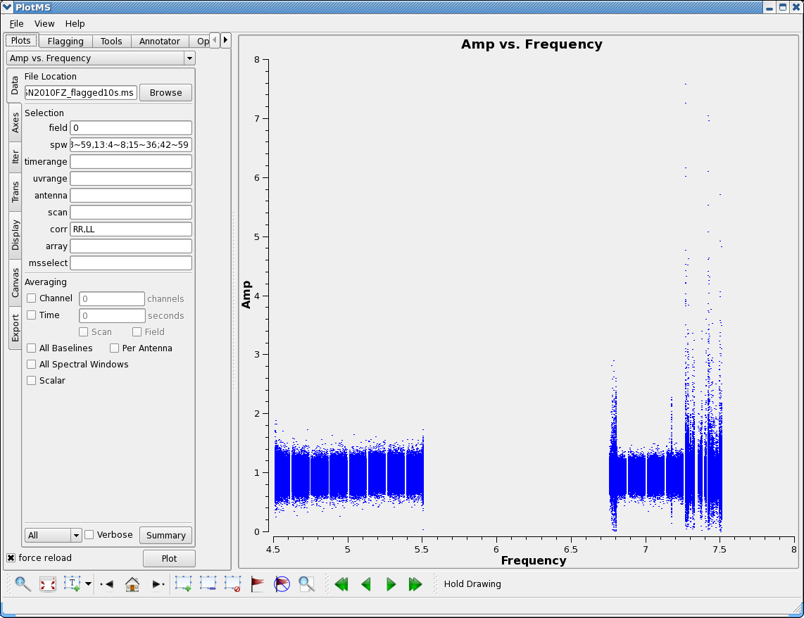
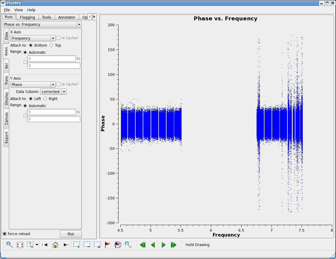
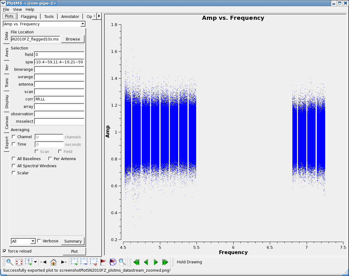
This now looks clean except for the RFI in the upper subbands.
Do flagging based on these:
# In CASA
flaglist2 = ['antenna="ea14,ea16,ea17,ea25" spw="5~7"']
flagcmd(vis='SN2010FZ_flagged10s.ms',inpmode='list',inpfile=flaglist2,action='apply')
Now replot the corrected data (you may have to force reload if you plotted same thing right before this):
# In CASA
plotms(vis='SN2010FZ_flagged10s.ms',field='2', \
       spw='0:10~59,1~7:4~59,8:4~13;18~59,9~11:4~59,12:4~13;18~29;31~33;46~51;53~59,13:4~8;15~36;42~59', \
       correlation='RR,LL',xaxis='frequency',yaxis='amp',ydatacolumn='corrected')
Looks pretty good.
Plot the phase:
# In CASA
plotms(vis='SN2010FZ_flagged10s.ms',field='2', \
       spw='0:10~59,1~7:4~59,8:4~13;18~59,9~11:4~59,12:4~13;18~29;31~33;46~51;53~59,13:4~8;15~36;42~59', \
       correlation='RR,LL',xaxis='frequency',yaxis='phase',ydatacolumn='corrected')
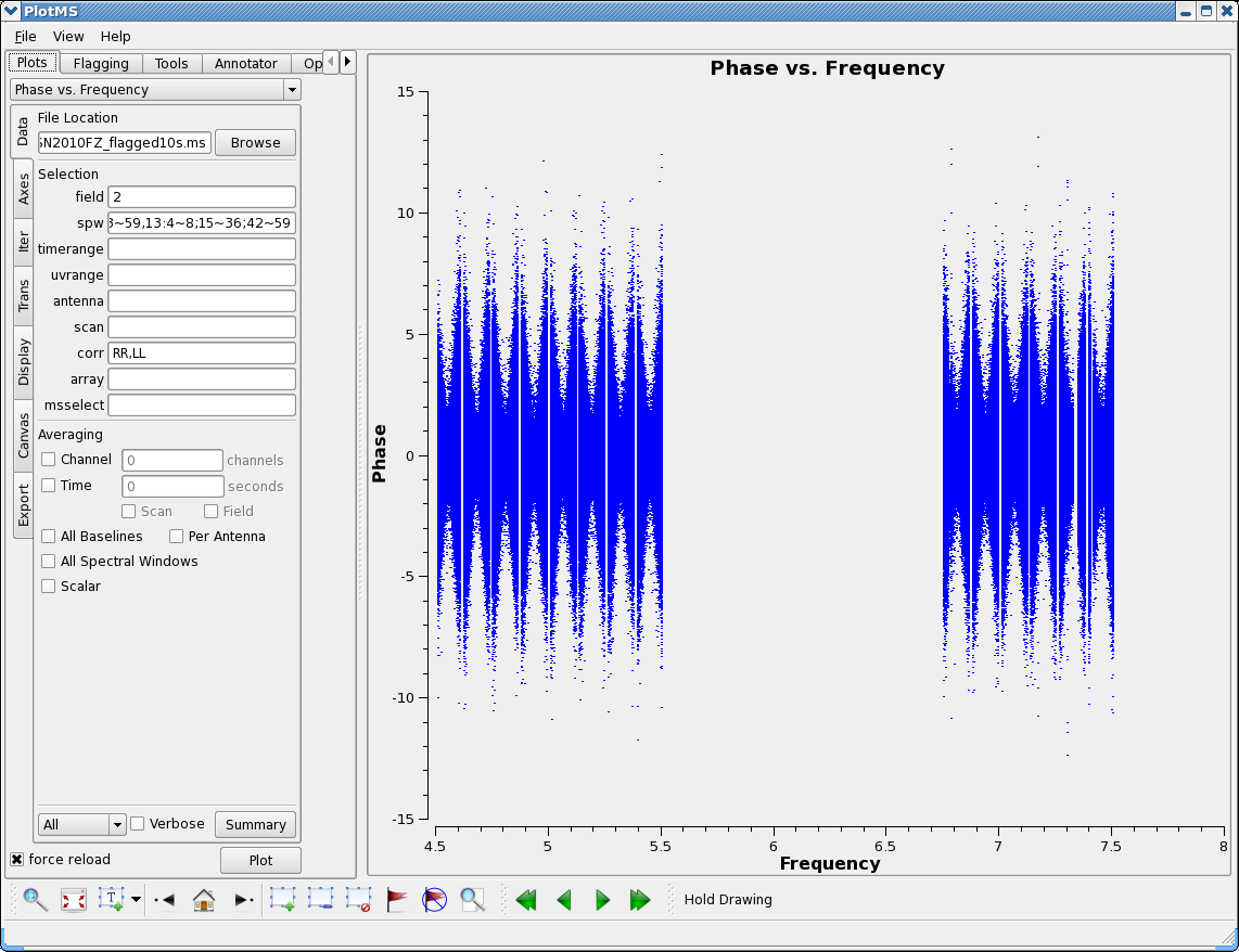
Note the characteristic "bowtie" pattern of the phases about the sub-band centers. Here we can see the effect of the EVLA "delay clunking", where the delay steps through discrete values such that the phase goes from -11deg to +11deg across the sub-band as the delay changes due to geometry. This is D-configuration so the delays change slowly, it will change faster in wider configurations. As of Q3 2011 we have not enabled the corrections for this in the EVLA system so you will always have this remaining delay error in your data. In principle, you could solve for delays on short timescales and take this out; in practice, this in not possible for your weaker science target source (where it would matter most for results).
Now let's plot the corrected data amplitude for the phase calibrator (field 0):
# In CASA
plotms(vis='SN2010FZ_flagged10s.ms',field='0', \
       spw='0:10~59,1~7:4~59,8:4~13;18~59,9~11:4~59,12:4~13;18~29;31~33;46~51;53~59,13:4~8;15~36;42~59', \
       correlation='RR,LL',xaxis='frequency',yaxis='amp',ydatacolumn='corrected')
You can see the bandpass filter roll-off increasing the noise at the baseband edges (about 8-16 channels worth). Also, we can see some RFI we missed:
- <6804 MHz spw 8 below ch 30 lots of bad stuff (a lot from ea18,ea22 but others too)
- 7168 MHz spw 11 ch 20
- pretty much all of spw 12,13
The ch 20 ones are all harmonics of a notorious 128 MHz tone. NOTE: You can get the frequency of a RFI feature by looking at the logger report from using the Locate ![]() tool.
tool.
We will not flag these, but exclude them in imaging (so that more advanced students can try flagging these in detail or using auto-flagging). A good channel selection string for imaging might be:
spw = '0:16~59,1~6:4~59,7:4~54,8:30~59,9~10:4~59,11:4~19;21~59'
Without further flagging, it may be best to drop spw 12-13 for imaging (we will do so from now on).
Plot again (including this selection for spw 0-11):
# In CASA
plotms(vis='SN2010FZ_flagged10s.ms',field='0', \
       spw='0:16~59,1~6:4~59,7:4~54,8:30~59,9~10:4~59,11:4~19;21~59', \
       correlation='RR,LL',xaxis='frequency',yaxis='amp',ydatacolumn='corrected')
Looks better.
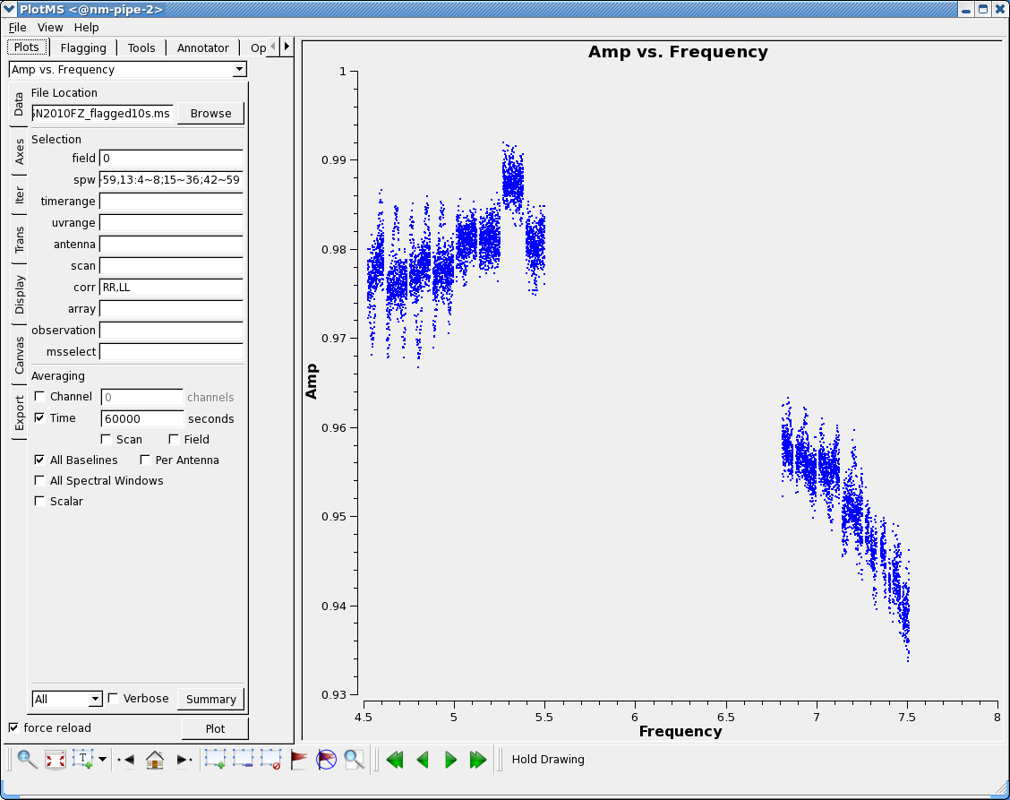
Now plot amplitudes for the corrected data averaged over baseline to see the source spectrum:
# In CASA
plotms(vis='SN2010FZ_flagged10s.ms',field='0',
       spw='0:16~59,1~6:4~59,7:4~54,8:30~59,9~10:4~59,11:4~19;21~59,12:4~13;18~29;31~33;46~51;53~59,13:4~8;15~36;42~59',
       correlation='RR,LL',avgbaseline=True,avgtime='60000s',
       xaxis='frequency',yaxis='amp',ydatacolumn='corrected',
       customsymbol=True,symbolshape='circle',symbolsize=2)
The "custom" plotting parameters show how to control the symbol shape and size from the task.
The last two sub-bands spw 12-13 give reasonable values, with only a tiny offset from spw 8-11. There are also strange amplitude excursions, particularly in the low end of the first baseband. These must be coming from one or more scans. You can iterate over scan to see the strange amplitudes (mostly from scan 7):
# In CASA
plotms(vis='SN2010FZ_flagged10s.ms',field='0',
       spw='0:16~59,1~6:4~59,7:4~54,8:30~59,9~10:4~59,11:4~19;21~59,12:4~13;18~29;31~33;46~51;53~59,13:4~8;15~36;42~59',
       correlation='RR,LL',avgbaseline=True,avgtime='600s',iteraxis='scan',
       xaxis='frequency',yaxis='amp',ydatacolumn='corrected',
       customsymbol=True,symbolshape='circle',symbolsize=2)
Also, there is an offset with the amplitudes for spw 6, perhaps due to the problem with baseline ea17&ea25 (which we flagged, but didn't recalibrate afterward) and likely affected the fluxscale solution. This is troubling enough that we will quickly go through a second round of calibration.
A Quick Recalibration
We now go back and recalibrate the data. We may as well flag scan 7 first, as well:
# In CASA
flagdata(vis='SN2010FZ_flagged10s.ms', scan='7')
#
# Clear the corrected data and model from header
clearcal('SN2010FZ_flagged10s.ms',addmodel=False)
#
chanStr = '0:16~59,1~6:4~59,7:4~54,8:30~59,9~10:4~59,11:4~19;21~59'
#
mysetjy2 = setjy(vis='SN2010FZ_flagged10s.ms', field='2', scalebychan=True, modimage='3C286_C.im')
#
gaincal(vis='SN2010FZ_flagged10s.ms',caltable='calSN2010FZ.G0.2',field='2',spw='0~11:23~28',
        gaintable=['calSN2010FZ.antpos','calSN2010FZ.gaincurve'],
        gaintype='G',refant='ea04',calmode='p',solint='int',minsnr=3)
#
gaincal(vis='SN2010FZ_flagged10s.ms',caltable='calSN2010FZ.K0.2',
        gaintable=['calSN2010FZ.antpos','calSN2010FZ.gaincurve','calSN2010FZ.G0.2'],
        field='2', spw=chanStr, gaintype='K',
        refant='ea04', combine='scan', solint='inf', minsnr=3)
#
bandpass(vis='SN2010FZ_flagged10s.ms',caltable='calSN2010FZ.B0.2',
         gaintable=['calSN2010FZ.antpos','calSN2010FZ.gaincurve',
                    'calSN2010FZ.G0.2','calSN2010FZ.K0.2'],
         field='2',refant='ea04',solnorm=False,
         spw='0~11',
         bandtype='B', combine='scan', solint='inf')
#
gaincal(vis='SN2010FZ_flagged10s.ms',caltable='calSN2010FZ.G1.2int',
        gaintable=['calSN2010FZ.antpos','calSN2010FZ.gaincurve',
                   'calSN2010FZ.K0.2','calSN2010FZ.B0.2'],
        field='2',refant='ea04',solnorm=F,
        spw=chanStr,
        solint='int',gaintype='G',calmode='p')
#
gaincal(vis='SN2010FZ_flagged10s.ms',caltable='calSN2010FZ.G1.2int',
        gaintable=['calSN2010FZ.antpos','calSN2010FZ.gaincurve',
                   'calSN2010FZ.K0.2','calSN2010FZ.B0.2'],
        field='0',refant='ea04',solnorm=F,
        spw=chanStr,
        solint='int',gaintype='G',calmode='p',append=True)
#
gaincal(vis='SN2010FZ_flagged10s.ms',caltable='calSN2010FZ.G1.2inf',
        gaintable=['calSN2010FZ.antpos','calSN2010FZ.gaincurve',
                   'calSN2010FZ.K0.2','calSN2010FZ.B0.2'],
        field='0',refant='ea04',solnorm=F,
        spw=chanStr,
        solint='inf',gaintype='G',calmode='p')
#
gaincal(vis='SN2010FZ_flagged10s.ms', caltable='calSN2010FZ.G2.2',
        gaintable=['calSN2010FZ.antpos','calSN2010FZ.gaincurve',
                   'calSN2010FZ.K0.2','calSN2010FZ.B0.2','calSN2010FZ.G1.2int'],
        gainfield=['','','2','2','2'],
        interp=['','','nearest','nearest','nearest'],
        field='2',refant='ea04',solnorm=F,
        spw=chanStr,
        solint='inf',combine='scan',gaintype='G',calmode='a')
#
gaincal(vis='SN2010FZ_flagged10s.ms', caltable='calSN2010FZ.G2.2',
        gaintable=['calSN2010FZ.antpos','calSN2010FZ.gaincurve',
                   'calSN2010FZ.K0.2','calSN2010FZ.B0.2','calSN2010FZ.G1.2int'],
        gainfield=['','','2','2','0'],
        interp=['','','nearest','nearest','nearest'],
        field='0',refant='ea04',solnorm=F,
        spw=chanStr,
        solint='inf',gaintype='G',calmode='a',append=True)
#
gaincal(vis='SN2010FZ_flagged10s.ms', caltable='calSN2010FZ.G2.3',
        gaintable=['calSN2010FZ.antpos','calSN2010FZ.gaincurve',
                   'calSN2010FZ.K0.2','calSN2010FZ.B0.2','calSN2010FZ.G1.2int'],
        gainfield=['','','2','2','2'],
        interp=['','','nearest','nearest','nearest'],
        field='2',refant='ea04',solnorm=F,
        spw=chanStr,
        solint='inf',combine='scan',gaintype='G',calmode='a')
#
gaincal(vis='SN2010FZ_flagged10s.ms', caltable='calSN2010FZ.G2.3',
        gaintable=['calSN2010FZ.antpos','calSN2010FZ.gaincurve',
                   'calSN2010FZ.K0.2','calSN2010FZ.B0.2','calSN2010FZ.G1.2int'],
        gainfield=['','','2','2','0'],
        interp=['','','nearest','nearest','nearest'],
        field='0',refant='ea04',solnorm=F,
        spw=chanStr,
        solint='inf',combine='scan',gaintype='G',calmode='a',append=True)
#
myflux2 = fluxscale(vis='SN2010FZ_flagged10s.ms',caltable='calSN2010FZ.G2.3',
                    fluxtable='calSN2010FZ.F2.3inc',reference='2',transfer='0',
                    incremental=True)
#
applycal(vis='SN2010FZ_flagged10s.ms',field='2',spw='0~11',
         gaintable=['calSN2010FZ.antpos','calSN2010FZ.gaincurve','calSN2010FZ.K0.2',
                    'calSN2010FZ.B0.2','calSN2010FZ.G1.2int','calSN2010FZ.G2.2'],
         gainfield=['','','','','2','2'],
         interp=['','','nearest','nearest','linear','nearest'],
         parang=False,calwt=False)
#
applycal(vis='SN2010FZ_flagged10s.ms',field='0',spw='0~11',
         gaintable=['calSN2010FZ.antpos','calSN2010FZ.gaincurve','calSN2010FZ.K0.2',
                    'calSN2010FZ.B0.2','calSN2010FZ.G1.2int','calSN2010FZ.G2.2',
                    'calSN2010FZ.F2.3inc'],
         gainfield=['','','','','0','0','0'],
         interp=['','','nearest','nearest','nearest','nearest',''],
         parang=False,calwt=False)
#
applycal(vis='SN2010FZ_flagged10s.ms',field='1',spw='0~11',
         gaintable=['calSN2010FZ.antpos','calSN2010FZ.gaincurve','calSN2010FZ.K0.2',
                    'calSN2010FZ.B0.2','calSN2010FZ.G1.2inf','calSN2010FZ.G2.2',
                    'calSN2010FZ.F2.3inc'],
         gainfield=['','','','','0','0','0'],
         interp=['','','nearest','nearest','linear','linear',''],
         parang=False,calwt=False)
Note that we have set the variable chanStr for our channel selection; this makes the task commands shorter and easier to read.
The fluxscale output this time around is slightly different to the last:
Found reference field(s): 3C286
Found transfer field(s):  J0925+0019
Flux density for J0925+0019 in SpW=0 (freq=4.488e+09 Hz) is: 0.978946 +/- 0.00284837 (SNR = 343.686, N = 50)
Flux density for J0925+0019 in SpW=1 (freq=4.616e+09 Hz) is: 0.978634 +/- 0.00264066 (SNR = 370.602, N = 50)
Flux density for J0925+0019 in SpW=2 (freq=4.744e+09 Hz) is: 0.980438 +/- 0.00251668 (SNR = 389.575, N = 50)
Flux density for J0925+0019 in SpW=3 (freq=4.872e+09 Hz) is: 0.980116 +/- 0.00255481 (SNR = 383.636, N = 50)
Flux density for J0925+0019 in SpW=4 (freq=5e+09 Hz) is: 0.982175 +/- 0.00230804 (SNR = 425.545, N = 50)
Flux density for J0925+0019 in SpW=5 (freq=5.128e+09 Hz) is: 0.979574 +/- 0.00269688 (SNR = 363.225, N = 42)
Flux density for J0925+0019 in SpW=6 (freq=5.256e+09 Hz) is: 0.980193 +/- 0.00271312 (SNR = 361.279, N = 42)
Flux density for J0925+0019 in SpW=7 (freq=5.384e+09 Hz) is: 0.98102 +/- 0.00249166 (SNR = 393.721, N = 42)
Flux density for J0925+0019 in SpW=8 (freq=6.744e+09 Hz) is: 0.962693 +/- 0.00282815 (SNR = 340.397, N = 48)
Flux density for J0925+0019 in SpW=9 (freq=6.872e+09 Hz) is: 0.960313 +/- 0.00285418 (SNR = 336.459, N = 48)
Flux density for J0925+0019 in SpW=10 (freq=7e+09 Hz) is: 0.957056 +/- 0.00303716 (SNR = 315.116, N = 48)
Flux density for J0925+0019 in SpW=11 (freq=7.128e+09 Hz) is: 0.953964 +/- 0.00378326 (SNR = 252.154, N = 48)
Flux density for J0925+0019 in SpW=12 is:  INSUFFICIENT DATA
Flux density for J0925+0019 in SpW=13 is:  INSUFFICIENT DATA
Fitted spectrum for J0925+0019 with fitorder=1: Flux density = 0.973376 +/- 0.00118872 (freq=5.52174 GHz)
    spidx=-0.0573991 +/- 0.00778736201
The source spectrum plot now looks somewhat better:
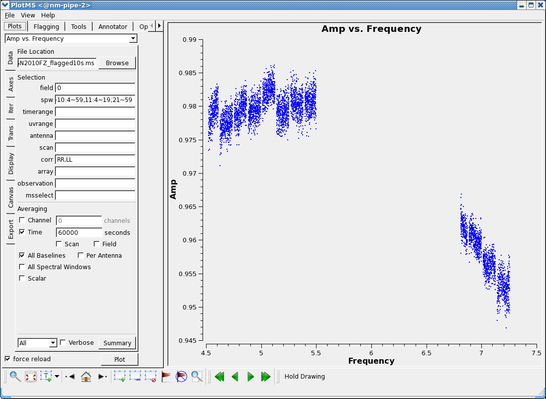
# In CASA
plotms(vis='SN2010FZ_flagged10s.ms',field='0', \
       spw='0:16~59,1~6:4~59,7:4~54,8:30~59,9~10:4~59,11:4~19;21~59', \
       correlation='RR,LL',avgbaseline=True,avgtime='60000s',
       xaxis='frequency',yaxis='amp',ydatacolumn='corrected',
       customsymbol=True,symbolshape='circle',symbolsize=2)
As you see in the figure to the right, there are still spectral window to window variations that deviate from a smooth spectrum. This is due to noise in the fluxscale median filter now used in CASA 4.0 (in this well-calibrated case, the old weighted means used by fluxscale in CASA3.4 behaved better). If we use plotcal to plot the solutions versus antenna
# In CASA
plotcal(caltable='calSN2010FZ.G2.3',xaxis='antenna',yaxis='amp',field='0',
        subplot=211,plotrange=[-1,-1,0.9,1.1])
plotcal(caltable='calSN2010FZ.G2.3',xaxis='antenna',yaxis='amp',field='2',
        subplot=212,plotrange=[-1,-1,0.9,1.1],figfile='plotSN2010FZ_plotcal_G2.3_ampant.png')
we see that there are variations that will enter into the medians. Some antennas are better behaved than others, for example ea12 (index 10) seems better than most.
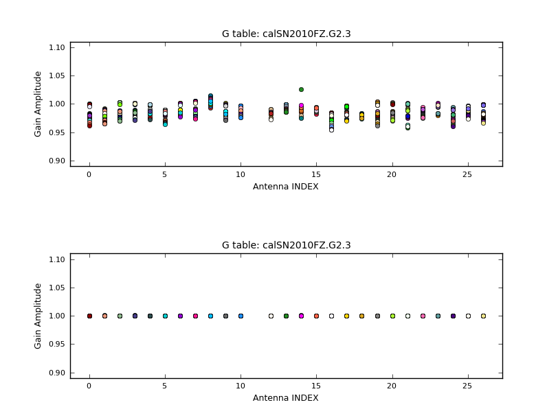
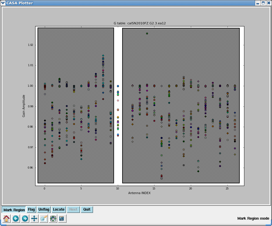
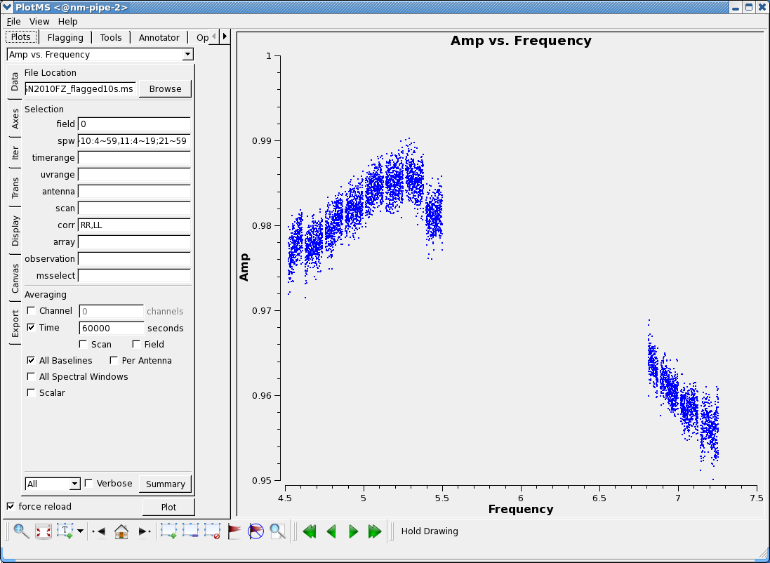
Because we are applying an incremental correction for the flux scale, we have the latitude to change the caltable that goes into fluxscale to get a better result. For example, we can restrict the antennas that are used to derive the scale. Although there is not yet antenna selection in fluxscale itself, we can edit the caltable using plotcal. For example, make a copy of the G2.3 caltable and select only a single antenna:
# In CASA
os.system('cp -rf calSN2010FZ.G2.3 calSN2010FZ.G2.3.ea12')
plotcal(caltable='calSN2010FZ.G2.3.ea12',xaxis='antenna',yaxis='amp')
In the plot to the right we show the GUI where we have boxed all but antenna ea12. Now we carry on with the fluxscale and applycal:
# In CASA
myfluxEdit3 = fluxscale(vis='SN2010FZ_flagged10s.ms',caltable='calSN2010FZ.G2.3.ea12',
                        fluxtable='calSN2010FZ.F2.3.ea12',reference='2',transfer='0',
                        incremental=True)
#
applycal(vis='SN2010FZ_flagged10s.ms',field='0',spw='0~11',
         gaintable=['calSN2010FZ.antpos','calSN2010FZ.gaincurve','calSN2010FZ.K0.2',
                    'calSN2010FZ.B0.2','calSN2010FZ.G1.2int','calSN2010FZ.G2.2',
                    'calSN2010FZ.F2.3.ea12'],
         gainfield=['','','','','0','0','0'],
         interp=['','','nearest','nearest','nearest','nearest',''],
         parang=False,calwt=False)
#
applycal(vis='SN2010FZ_flagged10s.ms',field='1',spw='0~11',
         gaintable=['calSN2010FZ.antpos','calSN2010FZ.gaincurve','calSN2010FZ.K0.2',
                    'calSN2010FZ.B0.2','calSN2010FZ.G1.2inf','calSN2010FZ.G2.2',
                    'calSN2010FZ.F2.3.ea12'],
         gainfield=['','','','','0','0','0'],
         interp=['','','nearest','nearest','linear','linear',''],
         parang=False,calwt=False)
The results appear better:
# In CASA
plotms(vis='SN2010FZ_flagged10s.ms',field='0', \
       spw='0:16~59,1~6:4~59,7:4~54,8:30~59,9~10:4~59,11:4~19;21~59', \
       correlation='RR,LL',avgbaseline=True,avgtime='60000s',
       xaxis='frequency',yaxis='amp',ydatacolumn='corrected',
       customsymbol=True,symbolshape='circle',symbolsize=2)
Note that if you choose a different antenna than ea12 to use for this, you will get different results, usually worse. But this procedure illustrates how to use the incremental solutions from fluxscale to your possible advantage.
We now return to examining our calibration.
We can also plot the corrected phase - looks good:
# In CASA
plotms(vis='SN2010FZ_flagged10s.ms',field='0', \
       spw='0:16~59,1~6:4~59,7:4~54,8:30~59,9~10:4~59,11:4~19;21~59', \
       correlation='RR,LL',xaxis='frequency',yaxis='phase',ydatacolumn='corrected')
We can average over baseline and each scan:
# In CASA
plotms(vis='SN2010FZ_flagged10s.ms',field='0', \
       spw='0:16~59,1~6:4~59,7:4~54,8:30~59,9~10:4~59,11:4~19;21~59', \
       correlation='RR,LL',avgbaseline=True,avgtime='600s',
       xaxis='frequency',yaxis='phase',ydatacolumn='corrected')
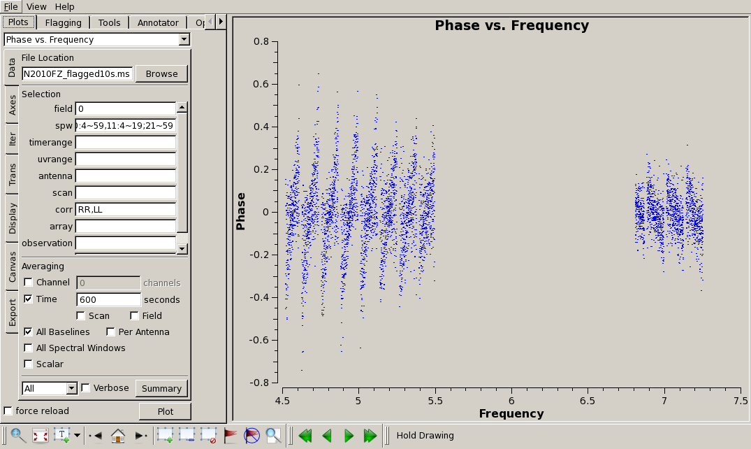
In this case, we can see the residual effect of the EVLA "delay clunking" described above, but it is reduced due to the averaging that we applied, but it is still there.
You can look at the target source field='1', but there are lots of data so you will need to do a lot of averaging. For example:
# In CASA
plotms(vis='SN2010FZ_flagged10s.ms',field='1',avgtime='300s', \
       spw='0:16~59,1~6:4~59,7:4~54,8:30~59,9~10:4~59,11:4~19;21~59', \
       correlation='RR,LL',xaxis='frequency',yaxis='amp',ydatacolumn='corrected')
Alas, the upper baseband still has lots of low level RFI.
Now split off the data for calibrators and target, to avoid later issues that can corrupt the MSs. We don't keep spw 12-15, since they weren't included in the last round of calibration, and we don't plan to image them.
# In CASA
# Remove any existing split data, otherwise split will not happen
os.system('rm -rf SN2010FZ_split10s.ms')
split(vis='SN2010FZ_flagged10s.ms',outputvis='SN2010FZ_split10s.ms', \
      datacolumn='corrected',field='1',spw='0~11')
#
# Remove any existing split data, otherwise split will not happen
os.system('rm -rf SN2010FZ_3c28610s.ms')
split(vis='SN2010FZ_flagged10s.ms',outputvis='SN2010FZ_3c28610s.ms', \
      datacolumn='corrected',field='2',spw='0~11')
#
# Remove any existing split data, otherwise split will not happen
os.system('rm -rf SN2010FZ_J092510s.ms')
split(vis='SN2010FZ_flagged10s.ms',outputvis='SN2010FZ_J092510s.ms', \
      datacolumn='corrected',field='0',spw='0~11')
Imaging
This is EVLA D-configuration data at C-band. To determine the best parameters for imaging, it helps to start with the relevant information in the Observational Status Summary:
- Synthesized beam should be 12" at 6 GHz with primary beam field of view of 7.5 arcmin (450")
Our data spans 4.5-7.5 GHz: this is a relatively large fractional bandwidth, resulting in substantial variation of the field of view over the entire frequency range. FOV = 45 arcmin / Frequency (GHz), giving 10 arcmin at 4.5 GHz, and 6 arcmin at 7.5 GHz. Likewise, the synthesized beam ranges from 16" at 4.5 GHz to 9.6" at 7.5 GHz. We want to subsample the synthesized beam by a factor of 3-4, so will use a cellsize of 3". To cover the full FOV (keeping it at the inner part of the image) at the lowest frequencies, we will want an image size of >400 pixels, or >20 arcmin.
We will also use the Briggs robust (with robust=0.5) weighting, which is a compromise between uniform and natural weighting, and will give reasonable resolution but will allow us to still see larger scale structure.
Due to the numerology of FFTW's (which clean uses under the hood for FFTs) optimal sizes, imsize should be composite number with two and only two prime factors chosen from 2, 3, and 5. Taking into account the x1.2 padding that clean uses internally to the imsize you give it (and 1.2 = 2*3/5), we choose 640 or 1280 as our imsize (640 = 2^7*5). Other reasonable sets would be 405, 1215, etc. (405 = 3^4*5) or 432, 648, 1296 (these are 2^n*3^m*5). In practice, if you give it non-optimal values for imsize, you may find that the transforms take a bit longer, which is noticeable if you are doing interactive clean.
WARNING: By default, a single-field nterms=1 clean does NOT use Cotton-Schwab (CS) clean to break into major cycles going back to data residuals, it just does cleaning in a bunch of minor cycles in the image plane. This can give much poorer imaging quality in cases with poor uv coverage (snapshots) or in the case of complex emission structure (like ours) -- clean tends to diverge in this case. You should explicitly set imagermode='csclean' in your call to clean. Also, in our case the psf is very good using mfs, so by default it will not take many major cycle breaks. We use the cyclefactor parameter to control this, which sets the break threshold to be cyclefactor times the max psf sidelobe level (outside the main peak). We start at cyclefactor=1.5 in a single spw, and ratchet it up to 4.5 when we clean all the spw. This seems to work ok. Rule of thumb is if it is gobbling up many hundreds of clean iterations in the minor cycles early on, increase cyclefactor. Conversely, if your psf is poor but you source structure is simple, you can reduce cyclefactor (e.g. below 1) to stop it from taking lots of extra major cycles.
For more information on using clean, in particular on using the interactive GUI, see EVLA_Continuum_Tutorial_3C391_CASA_4.2#Initial Imaging. WARNING: In CASA 4.0 the GUI interface for clean and the viewer has changed slightly. Some of the screenshots shown below may differ slightly from what you see.
NOTE: If you are pressed for time, then you might want to jump ahead to EVLA_6cmWideband_Tutorial_SN2010FZ_CASA_4.2#Cleaning_the_lower_baseband_using_two_MFS_Taylor_terms and while it is cleaning you can read the other Imaging descriptions.
Cleaning a single spectral window
Let us start by interactively cleaning one of the lower baseband spw (spw 5 in this example). NOTE: this first time will take a few minutes at start to create scratch columns in the MS in case we want to do self-calibration later.
Note that interrupting clean by Ctrl+C may corrupt your visibilities -- you may be better off choosing to let clean finish. We are currently implementing a command that will nicely exit to prevent this from happening, but for the moment try to avoid Ctrl+C.
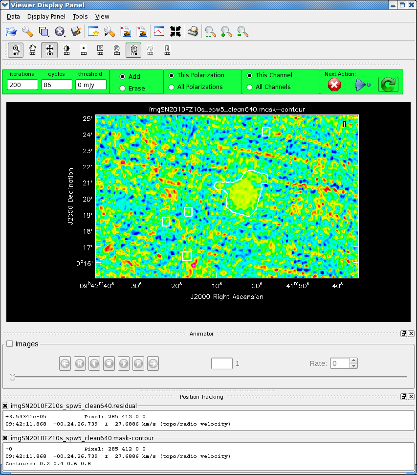
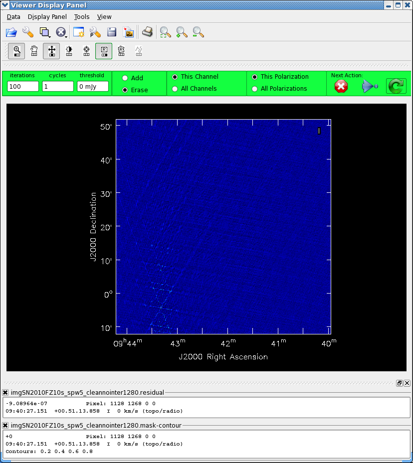
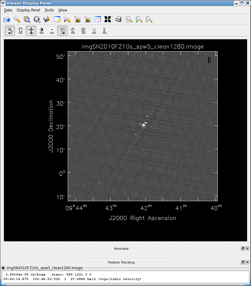
# In CASA
# Removing any previous cleaning information
# This assumes you want to start this clean from scratch
# If you want to continue this from a previous clean run,
# the rm -rf system command should be be skipped
os.system ('rm -rf imgSN2010FZ10s_spw5_clean640*')
clean(vis='SN2010FZ_split10s.ms',spw='5:4~59', \
      imagename='imgSN2010FZ10s_spw5_clean640', \
      mode='mfs',nterms=1,niter=10000,gain=0.1,threshold='0.0mJy', \
      psfmode='clark',imsize=[640,640],cell=['3.0arcsec'],stokes='I', \
      imagermode='csclean', cyclefactor=1.5, \
      weighting='briggs',robust=0.5,interactive=True)
- Start carefully by boxing the bright source and setting iterations to 10 at first
- Gradually add more boxes and increase the number of iterations
- Since this is not much more than a snapshot you see the six-fold sidelobe pattern
of the extended emission in the center of the map. This decreases as you clean out this emission.
- Stop cleaning when the residuals look like noise (and you cannot clearly see sources).
- To stop, click the red
 button.
The top figure to the right shows a zoom in on the end state of the clean, where we have marked a number of boxes and cleaned them out.
Note that there are some strange sidelobe patterns in lower left, possibly from a source outside the image area. We can make a bigger image starting from our current model:
# In CASA
# Removing any previous cleaning information
# This assumes you want to start this clean from scratch
# If you want to continue this from a previous clean run,
# the rm -rf system command should be skipped
os.system ('rm -rf imgSN2010FZ10s_spw5_clean1280*')
clean(vis='SN2010FZ_split10s.ms',spw='5:4~59', \
      imagename='imgSN2010FZ10s_spw5_clean1280', \
      mode='mfs',nterms=1,niter=10000,gain=0.1,threshold='0.0mJy', \
      psfmode='clark',imsize=[1280,1280],cell=['3.0arcsec'],stokes='I', \
      imagermode='csclean', cyclefactor=1.5, \
      modelimage='imgSN2010FZ10s_spw5_clean640.model', \
      weighting='briggs',robust=0.5,interactive=True)
Sure enough, there is a bright source near the lower left (see middle panel at right). Box it, clean it a bit, and look again. There is a second source in the mid-left (track it down by its sidelobes). Box this one, clean it a bit, and when satisfied stop.
You can use the CASA viewer to display the images that clean creates. If you need more guidance on using the viewer, see the CASA Viewer Demo video (note that this is for a much earlier version of the viewer, and the interface has changed since then).
Bring up your restored image directly:
# In CASA
viewer('imgSN2010FZ10s_spw5_clean1280.image')
The restored image is shown in the bottom panel to the right. I have chosen the Grayscale1 instead of default color map as I prefer "Grayscale" to false color "Rainbow" for assessing image quality. Also, you can change the scaling of the image using the "scaling power cycles" slider under "basic settings".
Check the rms of the residuals using the imstat task:
# In CASA
mystat = imstat('imgSN2010FZ10s_spw5_clean1280.residual')
print 'Residual standard deviation = '+str(mystat['sigma'][0])
In this particular case, it's 31.8 uJy; yours will likely be slightly different.
Cleaning the lower baseband
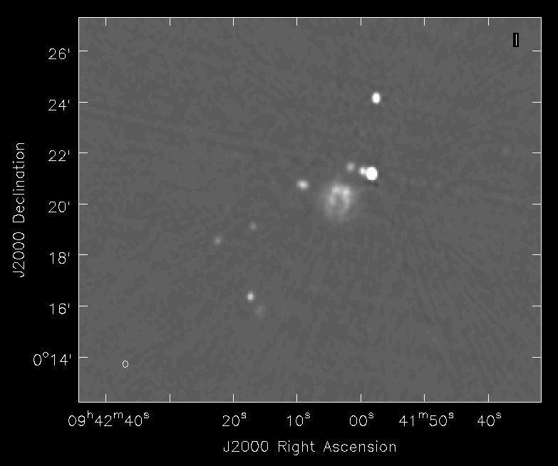
Now, image the entire lower baseband (spw 0-7). Follow same iterative procedure as before, and get the best residuals you can without "cleaning the noise".
- Because of the bandwidth and frequency synthesis, the sidelobe pattern is different than before and it is much easier to see fainter emission.
- Be careful cleaning sources that lie near or on sidelobe splotches.
- Clean the central emission region way down first to reduce the sidelobe level before adding components in the sidelobe areas.
# In CASA
# Removing any previous cleaning information
# This assumes you want to start this clean from scratch
# If you want to continue this from a previous clean run,
# the rm -rf system command should be be skipped
os.system ('rm -rf imgSN2010FZ10s_spw0to7_clean1280*')
clean(vis='SN2010FZ_split10s.ms',spw='0:16~59,1~6:4~59,7:4~54', \
      imagename='imgSN2010FZ10s_spw0to7_clean1280', \
      mode='mfs',nterms=1,niter=10000,gain=0.1,threshold='0.0mJy', \
      psfmode='clark',imsize=[1280,1280],cell=['3.0arcsec'],stokes='I', \
      imagermode='csclean', cyclefactor=1.5, \
      weighting='briggs',robust=0.5,interactive=True)
#
mystat = imstat('imgSN2010FZ10s_spw0to7_clean1280.residual')
print 'Residual standard deviation = '+str(mystat['sigma'][0])
For this run, the rms is 11.3 uJy (and there is clearly some structure left in the residual). To the right is a zoom-in on the center of the restored image.
Cleaning the lower baseband using two MFS Taylor terms
The mfs nterms=2 option creates two "Taylor Term" images - an average intensity image (with suffix .image.tt0) and a spectral slope image (with suffix .image.tt1) which is intensity x alpha (where alpha is spectral index). For convenience there is a spectral index image (with suffix .image.alpha). These Taylor expansions are with respect to the "Reference Frequency" of the image (by default the center frequency of the spw selected, but can be specified using the reffreq parameter in clean). The convention for spectral index alpha is that
[math]\displaystyle{ S \propto \nu^\alpha }[/math]
so negative spectral indexes indicate a "steep" spectrum (falling with frequency).

Let's try using multi-frequency synthesis with nterms=2 on the lower baseband. The dirty beam will have lower sidelobes so we turn up cyclefactor for csclean a bit. Note: if you're feeling a bit lazy, and trust your previous set of clean boxes, you can also set mask='imgSN2010FZ10s_spw0to7_clean1280.mask' to use these as a starting point:
# In CASA
# Removing any previous cleaning information
# This assumes you want to start this clean from scratch
# If you want to continue this from a previous clean run,
# the rm -rf system command should be be skipped
os.system ('rm -rf imgSN2010FZ10s_spw0to7_mfs2_clean1280*')
clean(vis='SN2010FZ_split10s.ms',spw='0:16~59,1~6:4~59,7:4~54', \
      imagename='imgSN2010FZ10s_spw0to7_mfs2_clean1280', \
      mode='mfs',nterms=2,niter=10000,gain=0.1,threshold='0.0mJy', \
      psfmode='clark',imsize=[1280,1280],cell=['3.0arcsec'],stokes='I', \
      imagermode='csclean', cyclefactor=4.5, \
      weighting='briggs',robust=0.5,interactive=True,mask=[])
#
mystat = imstat('imgSN2010FZ10s_spw0to7_mfs2_clean1280.residual.tt0')
print 'Residual standard deviation = '+str(mystat['sigma'][0])
For this run, the rms is 10.5 uJy (somewhat better-looking than the nterms=1). The top screenshot to the right shows an intermediate but early stage of cleaning where we are looking at the central emission and cleaning it out slowly.
You can use the viewer to load the average intensity image:
# In CASA
viewer('imgSN2010FZ10s_spw0to7_mfs2_clean1280.image.tt0')
and then use the Open Data panel to load the spectral index image imgSN2010FZ10s_spw0to7_mfs2_clean1280.image.alpha which can then be blinked (optionally plotted side-by-side using the Panel Display Options panel to set 2 panels in the x direction).
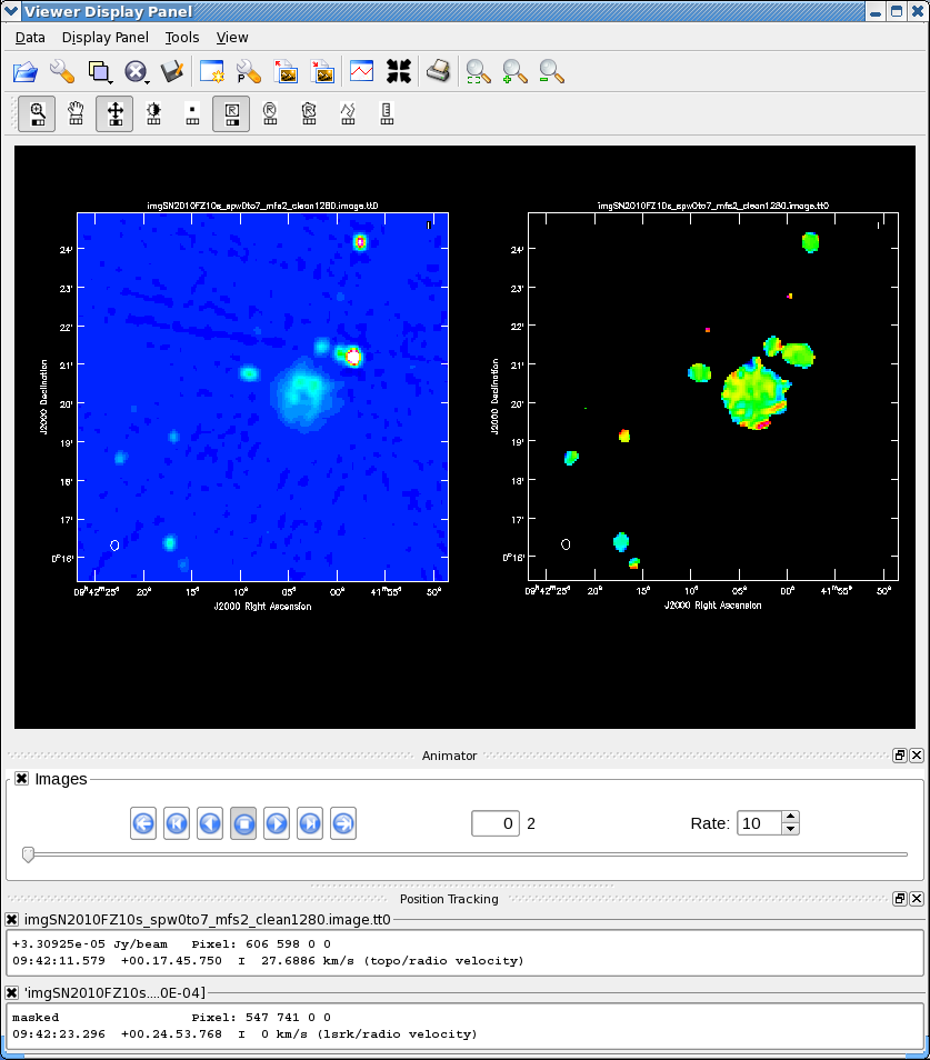
Note there is a lot of noise in alpha in the low-intensity regions, and thus filtering the alpha image based on the values in the tt0 image is desirable. You can use the immath task to make this filtered alpha image explicitly, using a Lattice Expression Language (LEL) expression:
# In CASA
immath(imagename=['imgSN2010FZ10s_spw0to7_mfs2_clean1280.image.alpha',
                  'imgSN2010FZ10s_spw0to7_mfs2_clean1280.image.tt0'],
       mode='evalexpr',
       expr='IM0[IM1>1.0E-4]',
       outfile='imgSN2010FZ10s_spw0to7_mfs2_clean1280.image.alpha.filtered')
This will use 0.1 mJy (or 10 x the sigma we found) as the cutoff. You can then view or manipulate the filtered alpha image as normal.
We can also use LEL to filter the alpha image on the intensity on-the-fly when we load this raster in the Open Data panel by specifying a LEL string in the LEL box instead of selecting the image from the directory listing. The LEL string:
'imgSN2010FZ10s_spw0to7_mfs2_clean1280.image.alpha'['imgSN2010FZ10s_spw0to7_mfs2_clean1280.image.tt0'>1.0E-04]
will replicate what we did above. The middle figure to the right shows the Open Data panel with our LEL string in it. Just click the Raster button to load this.
The lower panel to the right shows the intensity and LEL-filtered alpha images side-by-side in the viewer, zoomed in on the galaxy emission. Mousing over the alpha shows spectral indexes ranging from -1 to +1 in the center, with the brightest emission with alpha -0.7 in the knots in the disk.
Cleaning using both basebands combined
For the ultimate image, use the "clean" part of the upper baseband in addition to the lower (use spw 0-11). We will use mfs with nterms=2 (if you try nterms=1 on this wide bandwidth you will get much poorer residuals). Because of the added work and extra data involved, this will take much longer than our other runs of clean. Therefore, we will get a head start by doing a non-interactive clean using the mask left from the previous clean (spw 0-7). We will insert a clean threshold to limit runaway cleaning too far beneath the noise level.
This will take a while, especially if there are other processes running on your machine (with nothing else running, expect ~30-40 minutes).
# In CASA
# Removing any previous cleaning information
# This assumes you want to start this clean from scratch
# If you want to continue this from a previous clean run,
# the rm -rf system command should be be skipped
os.system ('rm -rf imgSN2010FZ10s_spw0to11_mfs2_clean1280*')
clean(vis='SN2010FZ_split10s.ms', \
      spw='0:16~59,1~6:4~59,7:4~54,8:30~59,9~10:4~59,11:4~19;21~59', \
      imagename='imgSN2010FZ10s_spw0to11_mfs2_clean1280', \
      mode='mfs',nterms=2,niter=3000,gain=0.1,threshold='0.002mJy', \
      psfmode='clark',imsize=[1280,1280],cell=['3.0arcsec'],stokes='I', \
      imagermode='csclean', cyclefactor=4.5, \
      mask=['imgSN2010FZ10s_spw0to7_mfs2_clean1280.mask'], \
      weighting='briggs',robust=0.5,interactive=False)
#
mystat = imstat('imgSN2010FZ10s_spw0to11_mfs2_clean1280.residual.tt0')
print 'Residual standard deviation = '+str(mystat['sigma'][0])
For this particular run, the rms was 8.9 uJy (noticeably better than the lower baseband only results).
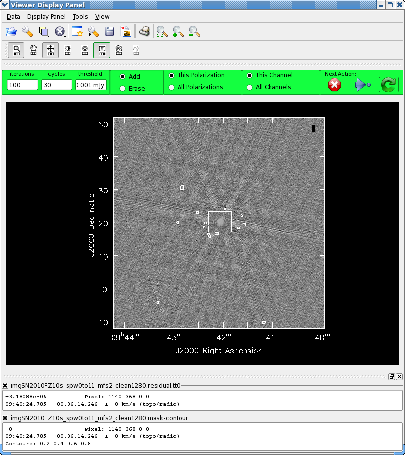
Let us see if there is more to clean. Bring this up in interactive mode:
# In CASA
clean(vis='SN2010FZ_split10s.ms', \
      spw='0:16~59,1~6:4~59,7:4~54,8:30~59,9~10:4~59,11:4~19;21~59', \
      imagename='imgSN2010FZ10s_spw0to11_mfs2_clean1280', \
      mode='mfs',nterms=2,niter=3000,gain=0.1,threshold='0.001mJy', \
      psfmode='clark',imsize=[1280,1280],cell=['3.0arcsec'],stokes='I', \
      imagermode='csclean', cyclefactor=4.5, \
      mask='imgSN2010FZ10s_spw0to11_mfs2_clean1280.mask', \
      weighting='briggs',robust=0.5,interactive=True)
This should start cleaning from where our previous non-interactive clean left off. Note for 4.2.0: In this case we have specified mask='imgSN2010FZ10s_spw0to11_mfs2_clean1280.mask' explicitly due to a bug where it will not otherwise allow you to edit the mask interactively.
You might find a few more sources revealed in the outer parts of the image, and also more emission around the galaxy disk in the center. Try drawing new boxes, perhaps extend the box in the center, and do ~100-1000 more iterations. At the end, what is left should be dominated by the error patterns from mis-calibration. Only self-calibration will get rid of these. Stop cleaning for now. See the figure to the right for the interactive display panel showing final residuals and mask (changing the colormap to Greyscale 1).
Check the residual levels:
# In CASA
mystat = imstat('imgSN2010FZ10s_spw0to11_mfs2_clean1280.residual.tt0')
sigma = mystat['sigma'][0]
print 'Residual standard deviation = '+str(mystat['sigma'][0])
The final rms achieved here is 8.7 uJy; slightly better.
Analyzing the image
Let's see how close we got to expected noise and dynamic range:
# In CASA
mystat = imstat('imgSN2010FZ10s_spw0to11_mfs2_clean1280.image.tt0')
peak = mystat['max'][0]
print 'Image max flux = '+str(mystat['max'][0])
#
mystat = imstat('imgSN2010FZ10s_spw0to11_mfs2_clean1280.model.tt0')
total = mystat['sum'][0]
print 'Model total flux = '+str(mystat['sum'][0])
#
snr = peak/sigma
print 'SN2010FZ peak S/N = '+str(snr)
#
snr = total/sigma
print 'SN2010FZ total S/N = '+str(snr)
The output gives:
Residual standard deviation = 8.74577600158e-06
Image max flux = 0.00993354152888
Model total flux = 0.0341279412654
SN2010FZ peak S/N = 1135.81019307
SN2010FZ total S/N = 3902.2199127
These are the numbers I got in my run-through. You may get slightly different values depending on how deeply you cleaned.
What do we expect? If we do listobs on this MS we see the scans:
  Date        Timerange (UTC)          Scan  FldId FieldName           nRows   Int(s)
  11-Jul-2010/21:38:44.0 - 21:39:51.0     9      0 SN2010FZ            33696  9.16
              21:40:01.0 - 21:41:20.5    10      0 SN2010FZ            37908  9.89
              21:41:30.0 - 21:42:50.0    11      0 SN2010FZ            37908  10
              21:43:00.0 - 21:44:20.0    12      0 SN2010FZ            37908  10
              21:44:30.0 - 21:45:50.0    13      0 SN2010FZ            37908  10
              21:46:00.0 - 21:47:19.5    14      0 SN2010FZ            37908  9.89
              21:47:29.0 - 21:47:49.0    15      0 SN2010FZ            12636  9.67
              21:49:42.0 - 21:50:49.0    17      0 SN2010FZ            33696  9.17
              21:50:59.0 - 21:52:19.0    18      0 SN2010FZ            37908  10
              21:52:29.0 - 21:53:48.5    19      0 SN2010FZ            37908  9.89
              21:53:58.0 - 21:55:18.0    20      0 SN2010FZ            37908  10
              21:55:28.0 - 21:56:48.0    21      0 SN2010FZ            37908  10
              21:56:58.0 - 21:58:18.0    22      0 SN2010FZ            37908  10
              21:58:28.0 - 21:58:47.5    23      0 SN2010FZ            12636  9.67
              22:00:39.5 - 22:01:47.0    25      0 SN2010FZ            33696  9.18
              22:01:57.0 - 22:03:17.0    26      0 SN2010FZ            37908  10
              22:03:27.0 - 22:04:47.0    27      0 SN2010FZ            37908  10
              22:04:57.0 - 22:06:16.5    28      0 SN2010FZ            37908  9.89
              22:06:26.0 - 22:07:46.0    29      0 SN2010FZ            37908  10
              22:07:56.0 - 22:09:16.0    30      0 SN2010FZ            37908  10
              22:09:26.0 - 22:09:45.5    31      0 SN2010FZ            12636  9.67
              22:11:38.0 - 22:12:45.5    33      0 SN2010FZ            33696  9.19
              22:12:55.0 - 22:14:15.0    34      0 SN2010FZ            37908  10
              22:14:25.0 - 22:15:45.0    35      0 SN2010FZ            37908  10
              22:15:55.0 - 22:17:15.0    36      0 SN2010FZ            37908  10
              22:17:25.0 - 22:18:44.5    37      0 SN2010FZ            37908  9.89
              22:18:54.0 - 22:20:14.0    38      0 SN2010FZ            37908  10
              22:20:24.0 - 22:20:43.5    39      0 SN2010FZ            12636  9.67
           (nVis = Total number of time/baseline visibilities per scan)
(listing columns truncated) and we estimate about 37 minutes on target. We had about 25 antennas on average, and our spw selection picked out 610 channels (2 MHz each) for a total of 1220 MHz bandwidth. If we plug this into the EVLA exposure calculator, at 5 GHz, we find that we expect a rms thermal noise level of 8.7 uJy, and at 7 GHz, 7.0 uJy. So, our values are within the expected range (a bit higher than theoretical, but that's expected).
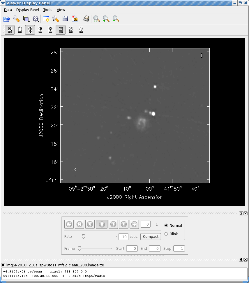
Look at this in the viewer:
# In CASA
viewer('imgSN2010FZ10s_spw0to11_mfs2_clean1280.image.tt0')
Zoom in on the center (see figure to the right).
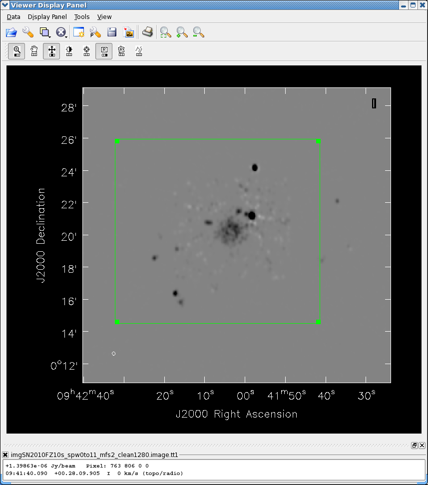
In the previous section we demonstrated how to process and display the spectral index image. You can do the same for this final image. Here, we will do some rough analysis on the spectral index to determine an intensity-weighted mean spectral index over the core region. The .image.tt1 from our mfs is an intensity times alpha image. See the figure to the right. Let's gate the Taylor-term images on intensity:
# In CASA
# Removing any file output from previous runs, so immath will proceed
os.system('rm -rf imgSN2010FZ10s_spw0to11_mfs2_clean1280.image.tt1.filtered')
immath(imagename=['imgSN2010FZ10s_spw0to11_mfs2_clean1280.image.tt1',
                  'imgSN2010FZ10s_spw0to11_mfs2_clean1280.image.tt0'],
       mode='evalexpr',
       expr='IM0[IM1>5.0E-5]',
       outfile='imgSN2010FZ10s_spw0to11_mfs2_clean1280.image.tt1.filtered')
#
# Removing any file output from previous runs, so immath will proceed
os.system('rm -rf imgSN2010FZ10s_spw0to11_mfs2_clean1280.image.tt0.filtered')
immath(imagename=['imgSN2010FZ10s_spw0to11_mfs2_clean1280.image.tt0'],
       mode='evalexpr',
       expr='IM0[IM0>5.0E-5]',
       outfile='imgSN2010FZ10s_spw0to11_mfs2_clean1280.image.tt0.filtered')
We can identify a box containing the central emission (see figure of tt1 in viewer) and note the corners. (We could also use the region tools from the viewer, but that is for another exercise.) Let us compute the intensity-weighted spectral index over this box by averaging these masked images using imstat and computing the ratio:
# In CASA
mystat = imstat('imgSN2010FZ10s_spw0to11_mfs2_clean1280.image.tt1.filtered',
                box='503,533,756,762')
avgtt0alpha = mystat['mean'][0]
#
mystat = imstat('imgSN2010FZ10s_spw0to11_mfs2_clean1280.image.tt0.filtered',
                box='503,533,756,762')
avgtt0 = mystat['mean'][0]
avgalpha = avgtt0alpha/avgtt0
print 'SN2010FZ I-weighted Alpha = '+str(avgalpha)
We get
SN2010FZ I-weighted Alpha = -1.38157453384
The emission in this source is on the steep side. At this point we do not know how reliable this is or what we expect (though our calibrators come out with correct spectral indexes if we image them the same way). But this illustrates a way to extract spectral information from our wideband mfs images.
Comparing with the Optical/Infrared
As a final comparison, we turn to the Sloan Digital Sky Survey (SDSS) and a cutout image of our galaxy:
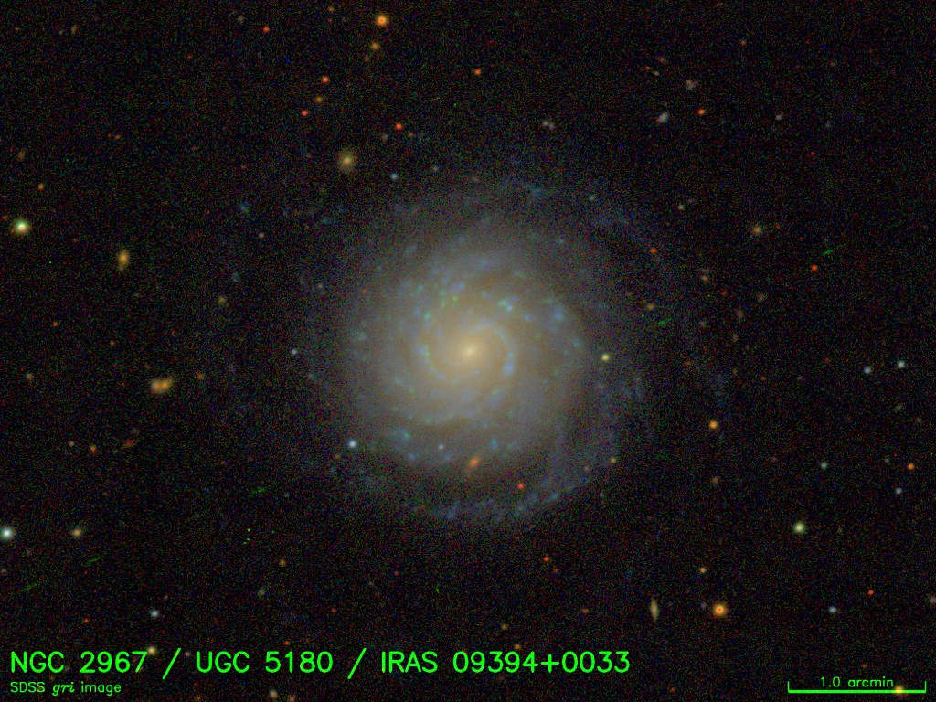
from their RC3 album (courtesy D.Hogg, M.Blanton, SDSS collaboration - see #Credits). This looks like a nice nearby face-on spiral galaxy. How does our 6cm continuum emission line up with the optical?
Here is the EVLA 6cm image side by side with a i-band image from the Sloan Digital Sky Survey (SDSS) registered to our image:
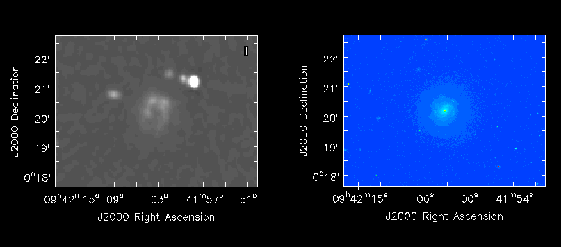
You can also find this image, named NGC_2967_UGC_5180_IRAS_09394+0033-i.fits, on the web at http://casa.nrao.edu/Data/EVLA/SN2010FZ/NGC_2967_UGC_5180_IRAS_09394+0033-i.fits (at the CASA workshop, it's in /data/casa/evla/ or a similar location that will be given to you in the instructions). Load it into your viewer, and blink against our 6cm image.
We can also plot one as a raster and the other overlaid as contours. You can load the SDSS image from the viewer Load Data panel and fiddle with contours. Once you know contour levels, you can also use the imview task to load a raster and contour image:
# In CASA
imview(raster={ 'file' : 'imgSN2010FZ10s_spw0to11_mfs2_clean1280.image.tt0'},
       contour = { 'file' : 'NGC_2967_UGC_5180_IRAS_09394+0033-i.fits',
                   'levels' : [0.2, 0.5, 1, 1.5, 3],
                   'base' : 0.0,
                   'unit' : 1.0 } )
The figure below shows the SDSS contours overlaid on our 6cm image (after fiddling with the colormap shift/slope for the EVLA raster image).
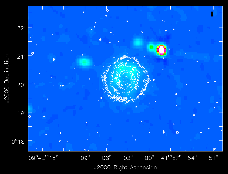
Likewise, we can plot the SDSS image as a raster and overlay EVLA 6cm contours:
# In CASA
imview(raster={ 'file' : 'NGC_2967_UGC_5180_IRAS_09394+0033-i.fits',
                'scaling' : -2.0,
                'range' : [0,10] },
       contour = { 'file' : 'imgSN2010FZ10s_spw0to11_mfs2_clean1280.image.tt0',
                   'levels' : [0.04, 0.08, 0.16, 0.32, 0.64, 1.28, 2.56],
                   'base' : 0.0,
                   'unit' : 0.001 },
       zoom = { 'blc' : [397,300],
                'trc' : [1567,1231] } )
This is shown in the figure below. Is the compact 6cm emission in upper left associated with a spiral arm?
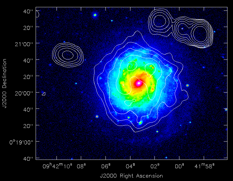
What to do next: some exercises for the user
Here are a number of things you can try after completing this tutorial:
- Use self-calibration to improve the data and re-clean to make a better image. See this tutorial for more information on self-calibration.
- Use multi-scale clean by adding non-zero scales to the multiscale parameter.
- Image the calibrators. What sort of dynamic range can you get on them? Is self-calibration needed (and if so what dynamic range do you get when you use it)?
- Try the testautoflag task (in 3.3.0 and later) to automatically flag RFI from the upper sideband. There is more information on running testautoflag in this tutorial.
Credits
The EVLA data was taken by A. Soderberg et al. as part of project AS1015. See NRAO eNews 3.8 (1-Sep-2010) for more on this result.
The Expanded Very Large Array (EVLA) is a partnership of the United States, Canada, and Mexico. The EVLA is funded in the United States by the National Science Foundation, in Canada by the National Research Council, and in Mexico by the Comisión Nacional de Investigación Científica y Tecnológica (CONICyT).
The National Radio Astronomy Observatory is a facility of the National Science Foundation operated under cooperative agreement by Associated Universities, Inc.
SDSS image courtesy David Hogg & Michael Blanton, private communication. Data comes from SDSS DR7, see Abazajian et. al 2009.
Funding for the SDSS and SDSS-II has been provided by the Alfred P. Sloan Foundation, the Participating Institutions, the National Science Foundation, the U.S. Department of Energy, the National Aeronautics and Space Administration, the Japanese Monbukagakusho, the Max Planck Society, and the Higher Education Funding Council for England. The SDSS Web Site is [1].
The SDSS is managed by the Astrophysical Research Consortium for the Participating Institutions. The Participating Institutions are the American Museum of Natural History, Astrophysical Institute Potsdam, University of Basel, University of Cambridge, Case Western Reserve University, University of Chicago, Drexel University, Fermilab, the Institute for Advanced Study, the Japan Participation Group, Johns Hopkins University, the Joint Institute for Nuclear Astrophysics, the Kavli Institute for Particle Astrophysics and Cosmology, the Korean Scientist Group, the Chinese Academy of Sciences (LAMOST), Los Alamos National Laboratory, the Max-Planck-Institute for Astronomy (MPIA), the Max-Planck-Institute for Astrophysics (MPA), New Mexico State University, Ohio State University, University of Pittsburgh, University of Portsmouth, Princeton University, the United States Naval Observatory, and the University of Washington.
Last checked on CASA Version 4.2.0.