CASA EVLA Scripts: Difference between revisions
No edit summary |
No edit summary |
||
| (29 intermediate revisions by 4 users not shown) | |||
| Line 1: | Line 1: | ||
[[Category:EVLA]] | [[Category:EVLA]] | ||
== Overview == | == Overview == | ||
This is a collection of Python scripts to help process and analyze EVLA data. Although they are not officially supported, some authors may choose to provide contact information. A brief description on how to run each script is provided by the author. If you would like to contribute, and do not have access to the CASA Guides Wiki, you may email | This is a collection of Python scripts to help process and analyze EVLA data. Although they are not officially supported, some authors may choose to provide contact information. A brief description on how to run each script is provided by the author. If you would like to contribute, and do not have access to the CASA Guides Wiki, you may email Juergen Ott (jott at nrao.edu). | ||
== Plotting the weather table, obtaining observation-specific opacity information == | == Plotting the weather table, obtaining observation-specific opacity information == | ||
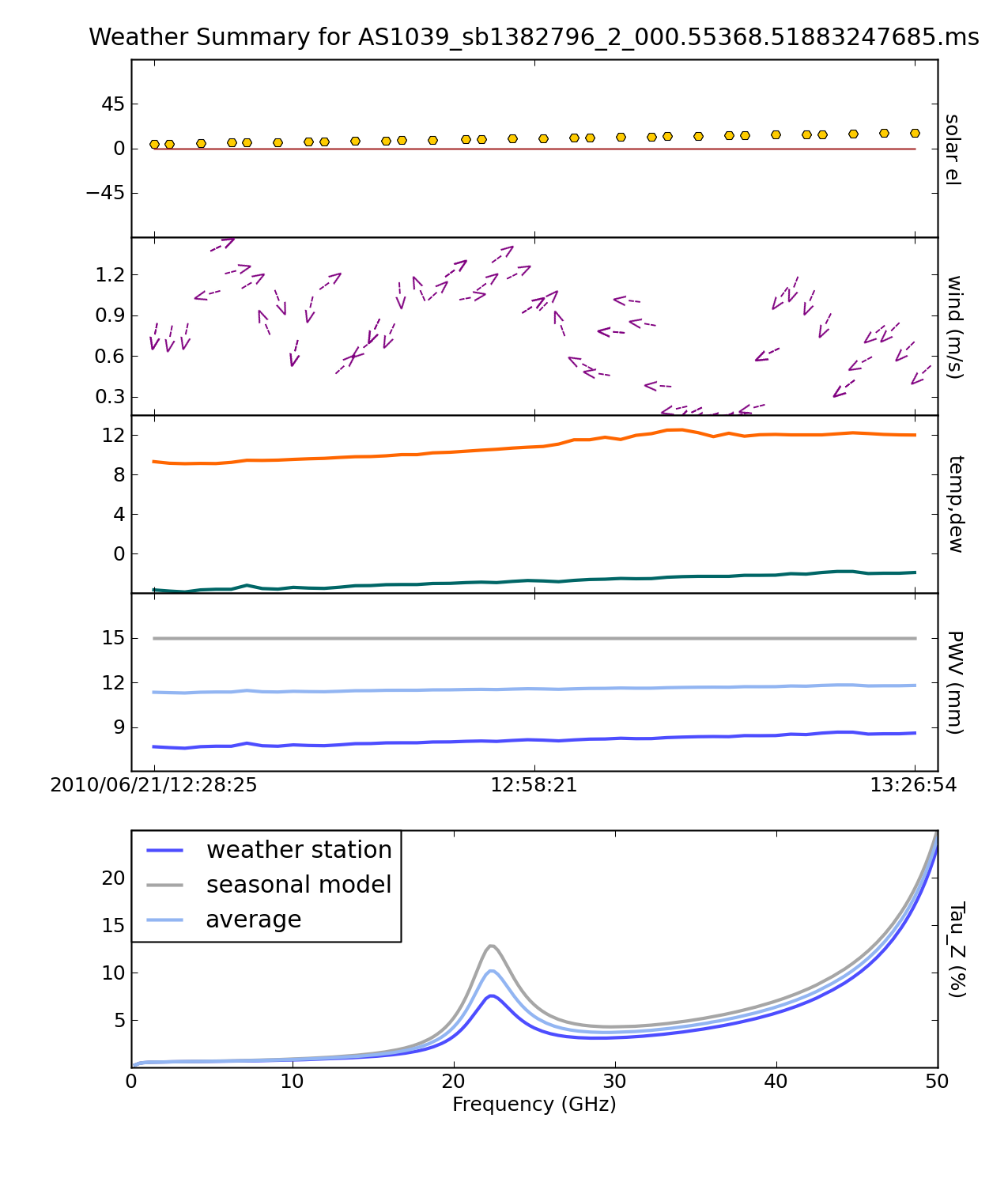
[[Image:PlotWX.png|200px|thumb|right|plotWX weather table figure]] | [[Image:PlotWX.png|200px|thumb|right|plotWX weather table figure]] | ||
<span style="color:#FF0000"> NOTE: A revised version of this method is now available in the CASA task 'plotweather'. Please use the new task for calibration purposes. </span> | |||
Download script: [[File:Script_plotWX.py]] | Download script: [[File:Script_plotWX.py]] | ||
| Line 32: | Line 31: | ||
#place Script_plotWX.py in your working directory | #place Script_plotWX.py in your working directory | ||
#open Script_plotWX.py in a text editor | #open Script_plotWX.py in a text editor | ||
# | #edit the last line of the script, replacing MSname.ms with the name of your measurement set, and save | ||
#in CASA, execute the script: | #in CASA, execute the script: | ||
| Line 54: | Line 52: | ||
</source> | </source> | ||
== | == Mosaicking Utilities == | ||
'''User beware: these are tested but not thoroughly vetted scripts provided without any guarantee.''' | |||
* Download script: [[File:buildmosaic.py]] | |||
* Download script: [[File:buildfluxmap.py]] | |||
* Download supporting module: [[File:axisutils.py]] | |||
* Download supporting module: [[File:constutils.py]] | |||
* Download supporting module: [[File:geoutils.py]] | |||
These are two potentially useful scripts ("buildmosaic" and "buildfluxmap") to aid in mosaic planning. A full-fledged GUI mosaic tool is under development by EVLA staff and RSRO participants but in the meantime these may be useful. They have been used but not heavily tested - please email aleroy at nrao dot edu to suggest improvements or report bugs. | |||
In fact an email to report use would be appreciated, if people actually use these I can simplify the dependencies (put everything in one file), wrap them up in the XML for a task, and strengthen the error-checking. | |||
The scripts are documented - please poke around to see more about the methodology or input parameters. | |||
=== buildmosaic === | |||
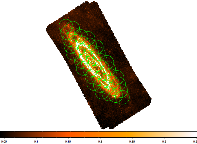
[[Image:Ds9_m31_1.png|200px|thumb|right|ds9 region output of "buildmosaic" overlaid on M31 IR map.]] | |||
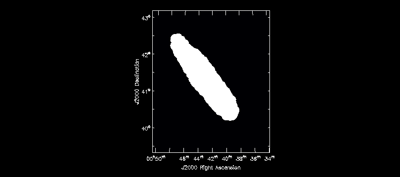
[[Image:M31_mask.png|200px|thumb|right|CASA viewer image of the mask "mask_m31.im" used to constrain the above mosaic.]] | |||
"buildmosaic" allows users to specify a hexagonally packed mosaic and then outputs this mosaic as a text file in one of three formats: EVLA proposal submission tool, simdata pointing file, or ds9 region file. "buildmosaic" is a python routine. To use it, make sure that "buildmosaic.py", "axisutils.py", "constutils.py", and "geoutils.py" all sit in your casapy path (the easiest way to do this is to just drop them into your working directory). Then type | |||
<source lang="python"> | <source lang="python"> | ||
# In CASA | # In CASA | ||
from | from buildmosaic import buildmosaic | ||
</source> | </source> | ||
then you can call "buildmosaic". Our test example was to build a large 2 GHz mosaic of M31 and the syntax we used to build this was something like this: | |||
<source lang="python"> | |||
# In CASA | |||
m31_dir = "00h42m44.3s +41d16m09s" | |||
buildmosaic(direction=m31_dir, | |||
format="evlapst", | |||
outfile="m31.pst", | |||
overwrite=True, | |||
freq=2.0e9, | |||
diam=25.0, | |||
posang=12.0, | |||
beamspacing=0.5, | |||
calcspacing=True, | |||
maxrad=10.0, | |||
mask="mask_m31.im", | |||
sourceroot="M31FIELD_", | |||
groupname="M31MOSAIC") | |||
</source> | |||
This | This long list of parameters tells "buildmosaic" how to build a hexagonally sampled mosaic - the center, spacing, orientation, and maximum extent - potentially subject to some spatial mask (an image of 1s and 0s, "buildmosaic" keeps only points coincident with a 1) and how to output the data to a text file. | ||
The options to specify the mosaic itself are: | |||
* "direction" specifies the center of the mosaic as a string. | |||
* "mask" supplies an optional CASA image containing only 1s and 0s. Only pointings inside the mask are kept (''this is an important feature!''). | |||
* "calcspacing" asks the program to calculate the spacing between mosaic points from the frequency and diameter of the telescope. | |||
** "freq" gives the observing frequency in Hz (used to calculate the primary beam). | |||
** "diam" gives the diameter of the telescope. | |||
** "beamspacing" dictates the spacing of pointing centers in units of the FWHM of the primary beam. | |||
* "spacing_deg" specifies the spacing in degrees (if you don't use "calcspacing"). | |||
* "posang" tilts the hexagonal pattern by this position angle. | |||
* "maxrad" gives the maximum distance from the center (in degrees) for a pointing to be considered. | |||
The ouput file is specified by | |||
* "outfile" specifies the text file output. | |||
** "overwrite" the file if present? | |||
** "format" specifies the output format ("evlapst", "simdata", or "ds9") of the output file. | |||
** "sourceroot", "groupname", etc. just feed to the output (specifically when using the PST format). Experiment to see these in use and have a look inside "buildmosaic.py" to see the other options that can be passed to a text file (a ds9 tag, velocity frame, etc.). | |||
=== buildfluxmap === | |||
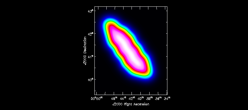
[[Image:m31_snr.png|200px|thumb|right|CASA viewer image of predicted signal-to-noise map of above mosaic.]] | |||
The second routine provided here gives a rough estimate of the sensitivity of a proposed mosaic. "buildfluxmap" accepts a template astrometry and a proposed mosaic and makes an image proportional to the expected signal-to-noise ratio. It does so by summing the square of the primary beam point by point and taking the square root of the resulting sum (see, e.g., Condon et al. 1998). "buildfluxmap" wants an input of the mosaic in ds9 format - this could be expanded if folks actually use it. | |||
The syntax is to provide it the proposed mosaic "ptgfile", a template image "template" that will be used as the astrometry for the signal to noise file, then to specify the observing frequency "freq" in Hz and telescope diameter "diam" in meters. | |||
<source lang="python"> | <source lang="python"> | ||
# In CASA | # In CASA | ||
from | from buildfluxmap import buildfluxmap | ||
buildfluxmap(ptgfile="m31_ds9.reg", | |||
template="mask_m31.im", | |||
outfile="snr_m31.im", | |||
freq=1.5e9, | |||
diam=25.0, | |||
overwrite=True) | |||
</source> | </source> | ||
== Align Two Cubes According to their Velocity Axes == | |||
'''Hopefully this will soon be deprecated by core CASA functionality. In the meantime please direct bug notes, suggestions, or just note use to aleroy at nrao dot edu.''' | |||
This is also planned future functionality for CASA but in the interim users working with multiple transitions or multiple observations of the same transition may find it desirable to align one cube so that its velocity axis matches that of another. This allows one to readily overlay the two cubes in the CASA viewer (which aligns data cubes by their spectral pixel rather than their velocity value). | |||
* Download script: [[File:alignbyvel.xml]] | |||
* Download script: [[File:alignbyvel.py]] | |||
* Download script: [[File:task_alignbyvel.py]] | |||
Download these scripts and follow the "buildmytasks" procedure described in the CASA Cookbook [http://casa.nrao.edu/docs/UserMan/UserManap7.html | here]. You can also access the functionality in python directly by importing task_alignbyvel.py. | |||
< | Once you have the task, simply pick a "template" cube that holds the desired velocity axis, an "infile" that holds the cube to be aligned, and specify an "outfile" to hold the output CASA image file. For example you could align the CN and CO images from the ALMA SV data on NGC 3256 like so: | ||
CASA | |||
<source lang="python"> | |||
# In CASA | |||
CN_im = 'n3256_CNlo.im/' | |||
CO_im = 'n3256_CO.im/' | |||
out = 'n3256_CNlo_to_CO.im/' | |||
alignbyvel(infile=CN_im, | |||
outfile=out, | |||
template=CO_im, | |||
overwrite=True) | |||
</source> | |||
</ | |||
Latest revision as of 15:40, 26 July 2013
Overview
This is a collection of Python scripts to help process and analyze EVLA data. Although they are not officially supported, some authors may choose to provide contact information. A brief description on how to run each script is provided by the author. If you would like to contribute, and do not have access to the CASA Guides Wiki, you may email Juergen Ott (jott at nrao.edu).
Plotting the weather table, obtaining observation-specific opacity information

NOTE: A revised version of this method is now available in the CASA task 'plotweather'. Please use the new task for calibration purposes.
Download script: File:Script plotWX.py
This script will plot weather information contained in the MS (see example below) as well as estimate the zenith opacity for each spectral window. This script is only intended for use with the EVLA-- it contains hardcoded site parameters and EVLA-specific models. Feel free to contact Josh Marvil (jmarvil + 'at' + nrao.edu) with questions or comments.
The plot will contain the following subfigures:
- The Sun's elevation, calculated from the date and time of the observation
- Wind speed and direction, as read from the weather table
- Temperature and Dewpoint, as read from the weather table
- Estimates of Precipitable Water Vapor (PWV), based upon:
- A Seasonal model based on VLA measurements between 1998-2005 (See VLA Test Memo #232)
- A calculation involving temperature and dewpoint (See VLA Scientific Memo #176)
- The average of the above two methods (currently accepted as the best predictor)
- Zenith optical depth from 1-50 GHz, calculated for each of the above three estimates of PWV, averaged over time. This calculation uses the atmospheric toolkit available within casa (see help(at) within CASA for more info)
This can be run from within CASA as a Script in the following way:
- place Script_plotWX.py in your working directory
- open Script_plotWX.py in a text editor
- edit the last line of the script, replacing MSname.ms with the name of your measurement set, and save
- in CASA, execute the script:
# In CASA
execfile 'Script_plotWX.py'
Or, this script can be run within CASA as a function:
- place Script_plotWX.py in your working directory
- in CASA, import the function definition and call the function, replacing MSname.ms with the name of your measurement set:
# In CASA
from Script_plotWX import plotWX
myTau = plotWX('MSname.ms')
Mosaicking Utilities
User beware: these are tested but not thoroughly vetted scripts provided without any guarantee.
- Download script: File:Buildmosaic.py
- Download script: File:Buildfluxmap.py
- Download supporting module: File:Axisutils.py
- Download supporting module: File:Constutils.py
- Download supporting module: File:Geoutils.py
These are two potentially useful scripts ("buildmosaic" and "buildfluxmap") to aid in mosaic planning. A full-fledged GUI mosaic tool is under development by EVLA staff and RSRO participants but in the meantime these may be useful. They have been used but not heavily tested - please email aleroy at nrao dot edu to suggest improvements or report bugs.
In fact an email to report use would be appreciated, if people actually use these I can simplify the dependencies (put everything in one file), wrap them up in the XML for a task, and strengthen the error-checking.
The scripts are documented - please poke around to see more about the methodology or input parameters.
buildmosaic


"buildmosaic" allows users to specify a hexagonally packed mosaic and then outputs this mosaic as a text file in one of three formats: EVLA proposal submission tool, simdata pointing file, or ds9 region file. "buildmosaic" is a python routine. To use it, make sure that "buildmosaic.py", "axisutils.py", "constutils.py", and "geoutils.py" all sit in your casapy path (the easiest way to do this is to just drop them into your working directory). Then type
# In CASA
from buildmosaic import buildmosaic
then you can call "buildmosaic". Our test example was to build a large 2 GHz mosaic of M31 and the syntax we used to build this was something like this:
# In CASA
m31_dir = "00h42m44.3s +41d16m09s"
buildmosaic(direction=m31_dir,
               format="evlapst",
               outfile="m31.pst",
               overwrite=True,
               freq=2.0e9,
               diam=25.0,
               posang=12.0,
               beamspacing=0.5,
               calcspacing=True,
               maxrad=10.0,
               mask="mask_m31.im",
               sourceroot="M31FIELD_",
               groupname="M31MOSAIC")
This long list of parameters tells "buildmosaic" how to build a hexagonally sampled mosaic - the center, spacing, orientation, and maximum extent - potentially subject to some spatial mask (an image of 1s and 0s, "buildmosaic" keeps only points coincident with a 1) and how to output the data to a text file.
The options to specify the mosaic itself are:
- "direction" specifies the center of the mosaic as a string.
- "mask" supplies an optional CASA image containing only 1s and 0s. Only pointings inside the mask are kept (this is an important feature!).
- "calcspacing" asks the program to calculate the spacing between mosaic points from the frequency and diameter of the telescope.
- "freq" gives the observing frequency in Hz (used to calculate the primary beam).
- "diam" gives the diameter of the telescope.
- "beamspacing" dictates the spacing of pointing centers in units of the FWHM of the primary beam.
- "spacing_deg" specifies the spacing in degrees (if you don't use "calcspacing").
- "posang" tilts the hexagonal pattern by this position angle.
- "maxrad" gives the maximum distance from the center (in degrees) for a pointing to be considered.
The ouput file is specified by
- "outfile" specifies the text file output.
- "overwrite" the file if present?
- "format" specifies the output format ("evlapst", "simdata", or "ds9") of the output file.
- "sourceroot", "groupname", etc. just feed to the output (specifically when using the PST format). Experiment to see these in use and have a look inside "buildmosaic.py" to see the other options that can be passed to a text file (a ds9 tag, velocity frame, etc.).
buildfluxmap

The second routine provided here gives a rough estimate of the sensitivity of a proposed mosaic. "buildfluxmap" accepts a template astrometry and a proposed mosaic and makes an image proportional to the expected signal-to-noise ratio. It does so by summing the square of the primary beam point by point and taking the square root of the resulting sum (see, e.g., Condon et al. 1998). "buildfluxmap" wants an input of the mosaic in ds9 format - this could be expanded if folks actually use it.
The syntax is to provide it the proposed mosaic "ptgfile", a template image "template" that will be used as the astrometry for the signal to noise file, then to specify the observing frequency "freq" in Hz and telescope diameter "diam" in meters.
# In CASA
from buildfluxmap import buildfluxmap
buildfluxmap(ptgfile="m31_ds9.reg",
                template="mask_m31.im",
                outfile="snr_m31.im",
                freq=1.5e9,
                diam=25.0,
                overwrite=True)
Align Two Cubes According to their Velocity Axes
Hopefully this will soon be deprecated by core CASA functionality. In the meantime please direct bug notes, suggestions, or just note use to aleroy at nrao dot edu.
This is also planned future functionality for CASA but in the interim users working with multiple transitions or multiple observations of the same transition may find it desirable to align one cube so that its velocity axis matches that of another. This allows one to readily overlay the two cubes in the CASA viewer (which aligns data cubes by their spectral pixel rather than their velocity value).
- Download script: File:Alignbyvel.xml
- Download script: File:Alignbyvel.py
- Download script: File:Task alignbyvel.py
Download these scripts and follow the "buildmytasks" procedure described in the CASA Cookbook | here. You can also access the functionality in python directly by importing task_alignbyvel.py.
Once you have the task, simply pick a "template" cube that holds the desired velocity axis, an "infile" that holds the cube to be aligned, and specify an "outfile" to hold the output CASA image file. For example you could align the CN and CO images from the ALMA SV data on NGC 3256 like so:
# In CASA
CN_im = 'n3256_CNlo.im/'
CO_im = 'n3256_CO.im/'
out = 'n3256_CNlo_to_CO.im/'
alignbyvel(infile=CN_im,
           outfile=out,
           template=CO_im,
           overwrite=True)