Plotconfig: Difference between revisions
No edit summary |
No edit summary |
||
| Line 3: | Line 3: | ||
This page documents the '''plotconfig''' function of Python module [[Analysis Utilities|analysisUtils]]. | This page documents the '''plotconfig''' function of Python module [[Analysis Utilities|analysisUtils]]. | ||
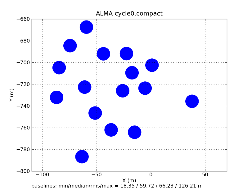
This function will make a plot of pad locations for any standard telescope configuration known to CASA (not limited to a specific observed ms). The size of the pad is equal to the diameter of the antenna. It also returns an array of the baseline lengths, sorted from shortest to longest. See also [[obslist]]. | This function will make a plot of pad locations for any standard telescope configuration known to CASA (not limited to a specific observed ms). The size of the pad is equal to the diameter of the antenna, unless the configuration is too large in which case there is a minimum marker size. It also returns an array of the baseline lengths, sorted from shortest to longest. See also [[obslist]]. | ||
==Usage== | ==Usage== | ||
Latest revision as of 15:47, 3 July 2013
Return to Analysis Utilities
This page documents the plotconfig function of Python module analysisUtils.
This function will make a plot of pad locations for any standard telescope configuration known to CASA (not limited to a specific observed ms). The size of the pad is equal to the diameter of the antenna, unless the configuration is too large in which case there is a minimum marker size. It also returns an array of the baseline lengths, sorted from shortest to longest. See also obslist.
Usage
au.plotconfig(telescope="", config="", figfile="", list=False, limits=None, gridlines=True, listconfig=False, cofa=[], title="")
telescope: name of the telescope (see below), or 'file'
config: name of the configuration for the specified telescope, or any user-supplied .cfg file if telescope='file'
figfile: a specific filename to give to the png (or True for automatic name generation)
gridlines: optional Boolean parameter to show dotted grid lines on major tick marks
limits: optional parameter for plot range: [x0,x1,y0,y1]
list: optional Boolean parameter to print the list of baseline lengths
listconfig: optional Boolean parameter to print the .cfg file
cofa: center-of-array coordinates [x,y,z]; if [], then use the value in CASA
title: title for plot (default is "telescope config")
Examples
Example 1. List the available telescopes and configurations.
# In CASA
au.plotconfig()
Telescope and configuration available to plot:
aca: i, ns, tp
alma: cycle0.compact, cycle0.extended, cycle1_1..6, 1..28
carma: a, b, c, d, e
meerkat
pdbi: a, b, c, d
sma: subcompact, compact, compact.n, extended, vextended
vla: a, bna, b, cnb, c, dnc, d
WSRT
Example 2. Plot the antenna pad locations for the ALMA Cycle 0 compact configuration.
# In CASA
CASA <3>: au.plotconfig('alma','cycle0.compact',figfile=True)
Read 16 pads
min/nextmin/median/mean/rms/max = 18.35 / 18.60 / 59.72 / 60.70 / 66.23 / 126.21 m
Wrote file = ALMA.cycle0.compact.png
  Out[3]:
array([  18.34928114,   18.59922814,   18.67225341,   19.68871438,
         20.7597779 ,   21.20105286,   21.3329793 ,   21.72915379,
         22.0800591 ,   22.59459018,   22.78237144,   25.78846509,
         25.83201484,   27.46895957,   27.49794209,   29.15634497,
         29.51343179,   31.55829422,   31.62250752,   32.54785378,
         34.38181744,   35.16912492,   35.18143753,   35.82266106,
         36.13044471,   36.45664452,   37.51364775,   38.35224408,
         38.35254654,   39.69908198,   40.3565153 ,   40.42755518,
         41.67060747,   41.96129664,   42.70404032,   44.19920722,
         44.904219  ,   44.98801461,   45.55421129,   45.93669031,
         46.3172296 ,   49.19301973,   49.30952918,   49.48707485,
         49.6219985 ,   49.69345204,   50.21704346,   51.29964177,
         52.43045363,   53.36047729,   53.43057901,   54.77903629,
         55.02455692,   55.24620569,   55.64613159,   55.95932051,
         58.43846541,   58.87265975,   59.35451767,   59.38838186,
         60.04523739,   61.13475674,   61.20365903,   61.79890065,
         61.99068325,   62.23888045,   62.24118429,   63.29582646,
         63.72437196,   63.80145741,   64.07662404,   64.59870677,
         65.21122832,   66.19442183,   67.23575586,   67.44667197,
         68.35948186,   69.82434388,   70.28085447,   70.35046477,
         70.4119276 ,   71.27848096,   71.58639724,   72.73992797,
         73.02277569,   74.6357243 ,   74.65195369,   75.88656385,
         77.55790771,   77.66319884,   77.94134408,   78.66300731,
         78.99645676,   79.3718099 ,   79.51404976,   81.32890711,
         81.89215932,   84.58133363,   85.51914888,   85.71695764,
         86.23846096,   89.81169974,   89.90704378,   91.43517893,
         92.5529028 ,   92.69516764,   96.68869426,   97.2890155 ,
         99.39936863,   99.74621451,  102.75273748,  103.30270508,
        106.0247318 ,  106.44602039,  113.42238358,  118.82496947,
        119.32132193,  123.42990694,  124.75264467,  126.21222105])
