Protoplanetary Disk Simulation (CASA 3.4): Difference between revisions
No edit summary |
|||
| (5 intermediate revisions by the same user not shown) | |||
| Line 2: | Line 2: | ||
[[Category: Simulations]] | [[Category: Simulations]] | ||
* '''This is an advanced simulation tutorial. New users are recommended to begin with the [[Simulation Guide for New Users (CASA 3.4)]].''' | |||
* '''This guide is applicable to CASA version 3.4. For older versions of CASA see [[PPdisk_simdata_(CASA_3.3)]].''' | * '''This guide is applicable to CASA version 3.4. For older versions of CASA see [[PPdisk_simdata_(CASA_3.3)]].''' | ||
* '''To create a script of the Python code on this page see [[Extracting scripts from these tutorials]].''' | * '''To create a script of the Python code on this page see [[Extracting scripts from these tutorials]].''' | ||
== Data == | == Data == | ||
| Line 27: | Line 26: | ||
</source> | </source> | ||
We now | We now use the '''ia''' (image analysis) and '''qa''' (units and quantities) tools from the CASA Toolkit to find the image center. In comparison to tasks, tools are a more advanced way of manipulating data in CASA. You can learn more about tools using the [http://casa.nrao.edu/docs/CasaRef/CasaRef.html tool reference manual]. | ||
When data are being manipulated with tools the data file must be explicitly opened and closed. | When data are being manipulated with tools the data file must be explicitly opened and closed. | ||
| Line 55: | Line 54: | ||
</source> | </source> | ||
Let's call our project "psim2". This defines the root prefix for any output files from simobserve. | |||
<source lang="python"> | <source lang="python"> | ||
project = "psim2" | |||
project | |||
</source> | </source> | ||
We'll set '''skymodel''' to the FITS file downloaded, above, and leave all '''skymodel''' subparameters at their default values. simobserve will create CASA image <tt>psim2.skymodel</tt>. | |||
<source lang="python"> | <source lang="python"> | ||
skymodel | skymodel = "input50pc_672GHz.fits" | ||
</source> | </source> | ||
We will specify the sky position for the center of the observation and set the map size to the size of the model image. Since the model image is 2/3 arcseconds across, we should only need one pointing. In this case, '''pointingspacing''' and '''maptype''' can be left at their default values. | |||
<source lang="python"> | <source lang="python"> | ||
setpointings = True | setpointings = True | ||
| Line 81: | Line 71: | ||
mapsize = "0.76arcsec" | mapsize = "0.76arcsec" | ||
</source> | </source> | ||
We do want to simulate an interferometric observation, so we set '''obsmode''' accordingly. We'll set '''totaltime''' to a 20-minute snapshot observation. | |||
<source lang="python"> | <source lang="python"> | ||
obsmode = "int" | obsmode = "int" | ||
| Line 89: | Line 79: | ||
</source> | </source> | ||
We want to use the appropriate antenna configuration for the desired angular resolution. Configuration 20, <tt>alma.out20.cfg</tt>, is the largest "compact" configuration. | |||
<source lang="python"> | <source lang="python"> | ||
antennalist = "alma.out20.cfg" | antennalist = "alma.out20.cfg" | ||
</source> | |||
Now run simobserve. | |||
<source lang="python"> | |||
simobserve() | simobserve() | ||
</source> | </source> | ||
Now that we've simulated the visibility measurements, we want to generate an image from the simulated data. '''simanalyze''' makes this easy. We begin by setting '''project''' to the same prefix used in simobserve and setting '''image''' to True. | |||
<source lang="python"> | <source lang="python"> | ||
default ("simanalyze") | default ("simanalyze") | ||
project | project = "psim2" | ||
image | image = True | ||
</source> | </source> | ||
We set '''modelimage''' to use the input FITS image when cleaning the simulated visibilities. We set the image size to 192 pixels square. | |||
<source lang="python"> | <source lang="python"> | ||
modelimage = "input50pc_672GHz.fits" | |||
vis = project + ".alma.out20.ms" | |||
imsize = [192, 192] | |||
</source> | </source> | ||
Specify the number of iterations for cleaning, with proper threshold and weighting. | |||
<source lang="python"> | <source lang="python"> | ||
niter = 10000 | |||
threshold = "1e-7Jy" | |||
weighting = "natural" | |||
</source> | </source> | ||
We'd like to calculate a difference and fidelity image, but we don't need to see the uv coverage. | |||
<source lang="python"> | <source lang="python"> | ||
showuv | analyze = True | ||
showresidual | showuv = False | ||
showconvolved | showresidual = True | ||
showconvolved = True | |||
</source> | </source> | ||
Plot both to the screen and PNG files with lots of messages. | |||
<source lang="python"> | <source lang="python"> | ||
graphics | graphics = "both" | ||
verbose | verbose = True | ||
overwrite = True | overwrite = True | ||
</source> | </source> | ||
Run simanalyze. | |||
<source lang="python"> | <source lang="python"> | ||
simanalyze() | simanalyze() | ||
</source> | </source> | ||
==Simulation Output== | |||
{| | {| cellspacing=2 | ||
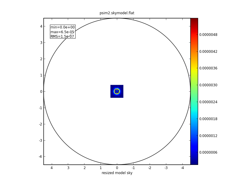
|Input:<br> [[File:Psim2.skymodel.png|300px]] | |Input:<br> [[File:Psim2.skymodel.png|300px]] | ||
| | |simobserve:<br> [[File:Psim2.alma.out20.observe.png|300px]] | ||
|- | |- | ||
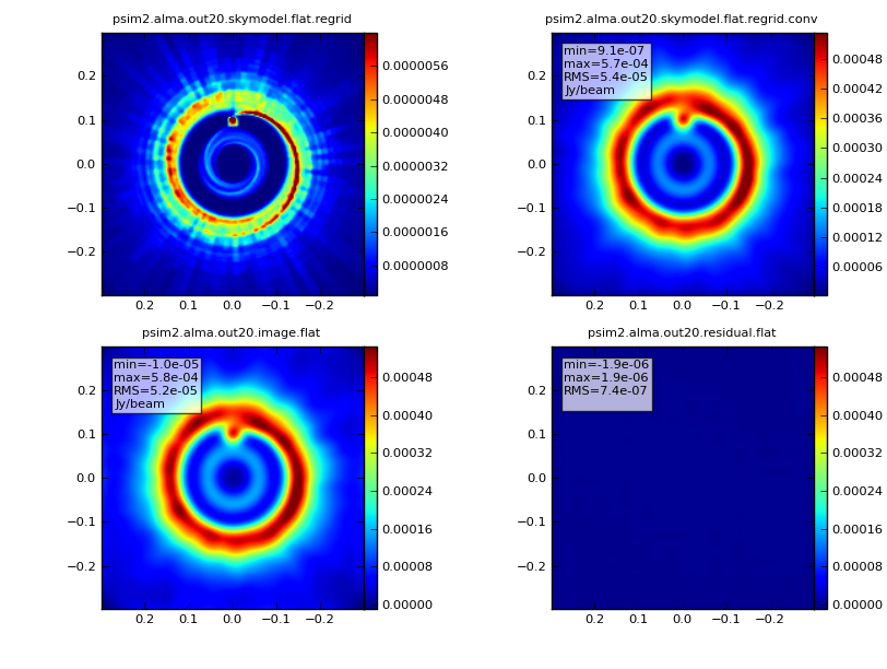
| | |simanalyze image:<br> [[File:Psim2.alma.out20.image.png|300px]] | ||
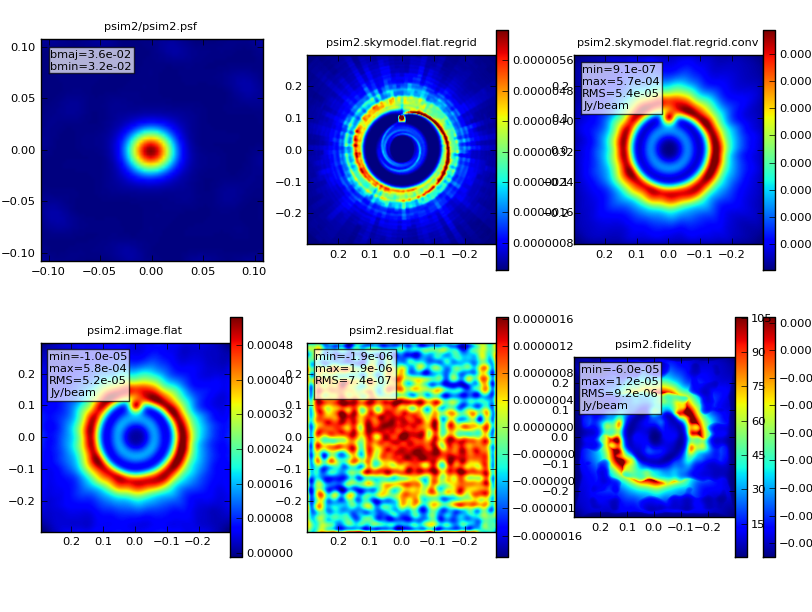
| | |simanalyze output:<br> [[File:Psim2.analysis.png|300px]] | ||
|} | |} | ||
{{Simulations Intro}} | {{Simulations Intro}} | ||
{{Checked 3.4.0}} | {{Checked 3.4.0}} | ||
Latest revision as of 19:37, 12 June 2012
↵ Simulating Observations in CASA
- This is an advanced simulation tutorial. New users are recommended to begin with the Simulation Guide for New Users (CASA 3.4).
- This guide is applicable to CASA version 3.4. For older versions of CASA see PPdisk_simdata_(CASA_3.3).
- To create a script of the Python code on this page see Extracting scripts from these tutorials.
Data
For this CASA Guide we will use a protoplanetary disk model from S. Wolf. If you use this FITS data for anything more than learning CASA, please cite Wolf & D'Angelo 2005.
Script with Explanation
Set simobserve as the current task and reset all parameters.
# In CASA
default("simobserve")
Review the image coordinate system using task imhead.
# This reports image header parameters in the Log Messages window
imhead("input50pc_672GHz.fits")
We now use the ia (image analysis) and qa (units and quantities) tools from the CASA Toolkit to find the image center. In comparison to tasks, tools are a more advanced way of manipulating data in CASA. You can learn more about tools using the tool reference manual.
When data are being manipulated with tools the data file must be explicitly opened and closed.
# In CASA
ia.open("input50pc_672GHz.fits")
Next, get the right ascension and declination of the image center. We get the number of pixels along each axis using ia.shape. Then, we get the RA and Dec values for the center pixel using ia.toworld.
# In CASA
axesLength = ia.shape()
# Divide the first two elements of axesLength by 2.
center_pixel = [ x / 2.0 for x in axesLength[:2] ]
# Feed center_pixel to ia.toworld and and save the RA and Dec to ra_radians and dec_radians
(ra_radians, dec_radians) = ia.toworld( center_pixel )['numeric'][:2]
ia.close()
Use the qa tool to convert the image center from radians to sexagesimal coordinates.
ra_hms  = qa.formxxx(str(ra_radians)+"rad",format='hms',prec=5)
dec_dms = qa.formxxx(str(dec_radians)+"rad",format='dms',prec=5)
Let's call our project "psim2". This defines the root prefix for any output files from simobserve.
project = "psim2"
We'll set skymodel to the FITS file downloaded, above, and leave all skymodel subparameters at their default values. simobserve will create CASA image psim2.skymodel.
skymodel = "input50pc_672GHz.fits"
We will specify the sky position for the center of the observation and set the map size to the size of the model image. Since the model image is 2/3 arcseconds across, we should only need one pointing. In this case, pointingspacing and maptype can be left at their default values.
setpointings       =  True
direction          =  "J2000 18h00m00.031s -22d59m59.6s"
mapsize            =  "0.76arcsec"
We do want to simulate an interferometric observation, so we set obsmode accordingly. We'll set totaltime to a 20-minute snapshot observation.
obsmode            =  "int"
totaltime          =  "1200s"
We want to use the appropriate antenna configuration for the desired angular resolution. Configuration 20, alma.out20.cfg, is the largest "compact" configuration.
antennalist = "alma.out20.cfg"
Now run simobserve.
simobserve()
Now that we've simulated the visibility measurements, we want to generate an image from the simulated data. simanalyze makes this easy. We begin by setting project to the same prefix used in simobserve and setting image to True.
default ("simanalyze")
project = "psim2"
image = True
We set modelimage to use the input FITS image when cleaning the simulated visibilities. We set the image size to 192 pixels square.
modelimage = "input50pc_672GHz.fits"
vis = project + ".alma.out20.ms"
imsize = [192, 192]
Specify the number of iterations for cleaning, with proper threshold and weighting.
niter = 10000
threshold = "1e-7Jy"
weighting = "natural"
We'd like to calculate a difference and fidelity image, but we don't need to see the uv coverage.
analyze = True
showuv = False
showresidual = True
showconvolved = True
Plot both to the screen and PNG files with lots of messages.
graphics = "both"
verbose = True
overwrite = True
Run simanalyze.
simanalyze()
Simulation Output
Input:
|
simobserve:
|
simanalyze image:
|
simanalyze output:
|
↵ Simulating Observations in CASA
Last checked on CASA Version 3.4.0.