Complex pointingtable (CASA 3.4): Difference between revisions
Created page with "blah" |
No edit summary |
||
| (2 intermediate revisions by the same user not shown) | |||
| Line 1: | Line 1: | ||
{{Simulations Intro}} | |||
[[Category: Simulations]] | |||
To create a script of the Python code on this page see [[Extracting scripts from these tutorials]]. | |||
simdata and simobserve can either generate mosaic pointing directions, or you can manually create a list. | |||
Then the directions are calculated for you, you are restricted to having the dwell time at each point in the mosaic be equal to the integration time parameter, i.e. the simulated ms will only have one timestamp per pointing or scan. This is not how real telescopes work, but simplifies the number of input parameters. If you want to do more complex things, for example 6s integrations in 5 min scans, or different integration times on different mosaic pointings, or a calibrator with a shorter integration time than the science pointings, the recommended method is to use simobserve to generate a simple pointing file (which is just an ascii file) and then edit it. | |||
We'll begin with simobserve, and use an Halpha image of M51 as a model, which you can download manually [[File:m51ha.fits.txt]] and place in your working directory, or use the curl command in the script: | |||
simobserve will make a copy m51c/m51c.skymodel, and not modify your input image. | |||
<source lang="python"> | |||
default "simobserve" | |||
project = "m51p" | |||
# Model sky = Halpha image of M51 | |||
os.system('curl http://casaguides.nrao.edu/images/3/3f/M51ha.fits.txt -f -o M51ha.fits.txt') | |||
skymodel = "M51ha.fits.txt" | |||
</source> | |||
Although the image has a world coordinate system, we want to override most of the parameters. | |||
* We'll place the source in the southern hemisphere with the indirection parameter, | |||
* set the pixel size to 0.1arcsec, effectively moving the galaxy further away (M51 itself would require a quite large mosaic, and in any case we need for the input model pixels to be significantly smaller than the synthesized beam that we'll be simulating, or else we won't be learning anything) | |||
* consistent with simulating a more distant source, we'll set the peak brightness to 0.004 Jy/pixel | |||
* set the frequency to 330GHz, and since its a 2D image we'll set the single "channel" width to be 50MHz, and peak brightness of 0.0004 Jy/pixel - parameters plausible for observing an emission line in a galaxy. | |||
<source lang="python"> | |||
# Set model image parameters: | |||
indirection="J2000 1h59m59.96s -34d59m59.50s" | |||
incell="0.1arcsec" | |||
inbright="0.0004" | |||
incenter="330.076GHz" | |||
inwidth="50MHz" | |||
</source> | |||
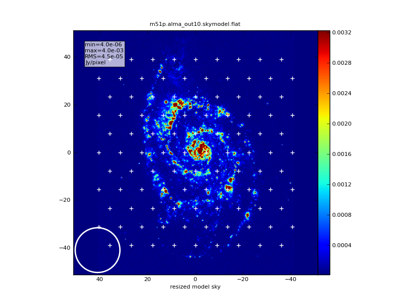
We'll begin with the 12m ALMA array observation, and have simobserve calculate a hexagonal mosaic of pointings. | |||
We'll set the integration time to 2min, since that's what we'll want for our scan duration or dwell time (if you ran observe with this parameter, as described above, you'd get one measurement every two minutes which would not result in realistic uv coverage). | |||
<source lang="python"> | |||
# have simobserve calculate mosaic pointing locations: | |||
setpointings = True | |||
integration = "2min" | |||
mapsize = "1.5arcmin" | |||
maptype = "hex" | |||
pointingspacing = "9arcsec" # this could also be specified in units of the primary beam e.g. "0.5PB" | |||
</source> | |||
Note that we're turning observe=False - we don't want to actually do the calculation (yet). | |||
<source lang="python"> | |||
obsmode = '' | |||
graphics = "both" | |||
go() | |||
</source> | |||
---- | |||
==== Edit Pointing File ==== | |||
[[Image:M51p.alma_out10.skymodel.png|thumb|hexagonal mosaic overplotted on sky model]] | |||
Open the pointing file created, m51p/m51p.alma_out10.ptg.txt, in a text editor. You'll see that it has a list of directions with dwell times in seconds: | |||
#Epoch RA DEC TIME | |||
J2000 02:59:57.03053 -034.59.20.528857 120.0 | |||
J2000 02:59:57.76290 -034.59.20.528857 120.0 | |||
J2000 02:59:58.49527 -034.59.20.528857 120.0 | |||
J2000 02:59:59.22763 -034.59.20.528857 120.0 | |||
... | |||
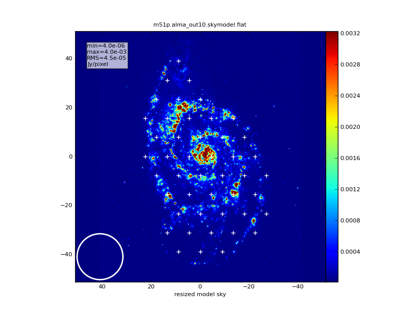
Let's delete the furthest east and west pointings, to make a more irregularly shaped map that covers only the galaxy. | |||
Also, we want to add a calibrator at 2:12:32.0 -30.10.04.0, observed every 10 minutes for 18 sec. | |||
The new file [[File:m51p.alma_out10.ptg.txt]] looks like | |||
#Epoch RA DEC TIME | |||
J2000 01:12:32.0 -030.10.04.0 18.0 | |||
J2000 02:00:00.69237 -034.59.20.528857 120.0 | |||
J2000 02:00:00.32619 -034.59.28.323085 120.0 | |||
J2000 02:00:01.05858 -034.59.28.323085 120.0 | |||
J2000 01:59:59.96000 -034.59.36.117314 120.0 | |||
J2000 02:00:00.69241 -034.59.36.117314 120.0 | |||
J2000 01:12:32.0 -030.10.04.0 18.0 | |||
J2000 02:00:01.42481 -034.59.36.117314 120.0 | |||
J2000 01:59:58.86136 -034.59.43.911543 120.0 | |||
J2000 01:59:59.59379 -034.59.43.911543 120.0 | |||
J2000 02:00:00.32621 -034.59.43.911543 120.0 | |||
J2000 02:00:01.05864 -034.59.43.911543 120.0 | |||
J2000 01:12:32.0 -030.10.04.0 18.0 | |||
J2000 02:00:01.79106 -034.59.43.911543 120.0 | |||
... | |||
Either download that file manually and place it in your m51p/ subdirectory (replacing the pointingfile that was just created in there), or use this curl command: | |||
<source lang="python"> | |||
os.system('curl http://casaguides.nrao.edu/images/4/44/M51p.alma_out10.ptg.txt -f -o m51p/m51p.alma_out10.ptg.txt') | |||
</source> | |||
[[Image:m51p.alma_out10b.skymodel.png|thumb|modified pointing file]] | |||
For our simulated calibrator, we want to create a point source componentlist, as described in [[Simulation_Guide_Component_Lists_(CASA_3.4)]]: | |||
<source lang="python"> | |||
# If m51p_cal.cl already exists, it needs to be deleted | |||
os.system('rm -rf m51p_cal.cl') | |||
cl.done() | |||
cl.addcomponent(dir="J2000 1h12m32.0s -30d10m04.0s", flux=0.9, fluxunit='Jy', freq='330.076GHz', shape="point") | |||
cl.rename('m51p_cal.cl') | |||
cl.close() | |||
</source> | |||
Note: there is a minor bug in CASAv16856 which will make the new pointings be plotted offset as in [[:Image:M51p.alma_out10.skymodel-offset.png]] - this is only a plotting issue; the simulation is calculated as expected with pointings on the galaxy. | |||
==== Observe irregular mosaic ==== | |||
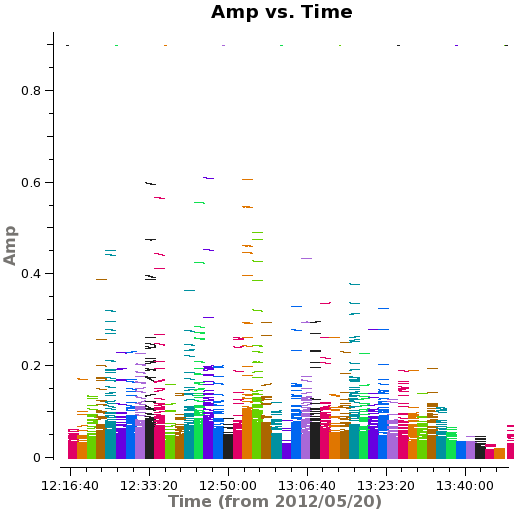
[[Image:m51p.amp.time.png|thumb|amplitude vs time, colored by field. The calibrator scans are visually apparent.]] | |||
Now run simobserve again, but with setpointings=False. We change the integration to 6s. simobserve will observe each pointing | |||
for the amount of time in the pointing file (we could have also changed the time on different pointings to be different), but with 6s integrations, resulting in 2min/6s data points per scan. | |||
We also add the calibrator componentlist. | |||
<source lang="python"> | |||
setpointings = False | |||
ptgfile = "m51p.alma_out10.ptg.txt" | |||
integration = "6s" | |||
# | |||
obsmode = 'int' | |||
complist = "m51p_cal.cl" | |||
totaltime = "2" | |||
</source> | |||
<source lang="python"> | |||
go() | |||
</source> | |||
Latest revision as of 13:32, 8 June 2012
↵ Simulating Observations in CASA
To create a script of the Python code on this page see Extracting scripts from these tutorials.
simdata and simobserve can either generate mosaic pointing directions, or you can manually create a list.
Then the directions are calculated for you, you are restricted to having the dwell time at each point in the mosaic be equal to the integration time parameter, i.e. the simulated ms will only have one timestamp per pointing or scan. This is not how real telescopes work, but simplifies the number of input parameters. If you want to do more complex things, for example 6s integrations in 5 min scans, or different integration times on different mosaic pointings, or a calibrator with a shorter integration time than the science pointings, the recommended method is to use simobserve to generate a simple pointing file (which is just an ascii file) and then edit it.
We'll begin with simobserve, and use an Halpha image of M51 as a model, which you can download manually File:M51ha.fits.txt and place in your working directory, or use the curl command in the script:
simobserve will make a copy m51c/m51c.skymodel, and not modify your input image.
default "simobserve"
project          =  "m51p"
# Model sky = Halpha image of M51
os.system('curl http://casaguides.nrao.edu/images/3/3f/M51ha.fits.txt -f -o M51ha.fits.txt')
skymodel         =  "M51ha.fits.txt"
Although the image has a world coordinate system, we want to override most of the parameters.
- We'll place the source in the southern hemisphere with the indirection parameter,
- set the pixel size to 0.1arcsec, effectively moving the galaxy further away (M51 itself would require a quite large mosaic, and in any case we need for the input model pixels to be significantly smaller than the synthesized beam that we'll be simulating, or else we won't be learning anything)
- consistent with simulating a more distant source, we'll set the peak brightness to 0.004 Jy/pixel
- set the frequency to 330GHz, and since its a 2D image we'll set the single "channel" width to be 50MHz, and peak brightness of 0.0004 Jy/pixel - parameters plausible for observing an emission line in a galaxy.
# Set model image parameters:
indirection="J2000 1h59m59.96s -34d59m59.50s"
incell="0.1arcsec"
inbright="0.0004"
incenter="330.076GHz"
inwidth="50MHz"
We'll begin with the 12m ALMA array observation, and have simobserve calculate a hexagonal mosaic of pointings.
We'll set the integration time to 2min, since that's what we'll want for our scan duration or dwell time (if you ran observe with this parameter, as described above, you'd get one measurement every two minutes which would not result in realistic uv coverage).
# have simobserve calculate mosaic pointing locations:
setpointings       =  True
integration        =  "2min"
mapsize            =  "1.5arcmin"
maptype            =  "hex"
pointingspacing    =  "9arcsec"      # this could also be specified in units of the primary beam e.g. "0.5PB"
Note that we're turning observe=False - we don't want to actually do the calculation (yet).
obsmode            =  ''
graphics           =  "both"
go()
Edit Pointing File

Open the pointing file created, m51p/m51p.alma_out10.ptg.txt, in a text editor. You'll see that it has a list of directions with dwell times in seconds:
#Epoch     RA          DEC      TIME
J2000 02:59:57.03053 -034.59.20.528857  120.0
J2000 02:59:57.76290 -034.59.20.528857  120.0
J2000 02:59:58.49527 -034.59.20.528857  120.0
J2000 02:59:59.22763 -034.59.20.528857  120.0
...
Let's delete the furthest east and west pointings, to make a more irregularly shaped map that covers only the galaxy. Also, we want to add a calibrator at 2:12:32.0 -30.10.04.0, observed every 10 minutes for 18 sec. The new file File:M51p.alma out10.ptg.txt looks like
#Epoch     RA          DEC      TIME
J2000 01:12:32.0     -030.10.04.0        18.0
J2000 02:00:00.69237 -034.59.20.528857  120.0
J2000 02:00:00.32619 -034.59.28.323085  120.0
J2000 02:00:01.05858 -034.59.28.323085  120.0
J2000 01:59:59.96000 -034.59.36.117314  120.0
J2000 02:00:00.69241 -034.59.36.117314  120.0
J2000 01:12:32.0     -030.10.04.0        18.0
J2000 02:00:01.42481 -034.59.36.117314  120.0
J2000 01:59:58.86136 -034.59.43.911543  120.0
J2000 01:59:59.59379 -034.59.43.911543  120.0
J2000 02:00:00.32621 -034.59.43.911543  120.0
J2000 02:00:01.05864 -034.59.43.911543  120.0
J2000 01:12:32.0     -030.10.04.0        18.0
J2000 02:00:01.79106 -034.59.43.911543  120.0
...
Either download that file manually and place it in your m51p/ subdirectory (replacing the pointingfile that was just created in there), or use this curl command:
os.system('curl http://casaguides.nrao.edu/images/4/44/M51p.alma_out10.ptg.txt -f -o m51p/m51p.alma_out10.ptg.txt')

For our simulated calibrator, we want to create a point source componentlist, as described in Simulation_Guide_Component_Lists_(CASA_3.4):
# If m51p_cal.cl already exists, it needs to be deleted
os.system('rm -rf m51p_cal.cl')
cl.done()
cl.addcomponent(dir="J2000 1h12m32.0s -30d10m04.0s", flux=0.9, fluxunit='Jy', freq='330.076GHz', shape="point")
cl.rename('m51p_cal.cl')
cl.close()
Note: there is a minor bug in CASAv16856 which will make the new pointings be plotted offset as in Image:M51p.alma_out10.skymodel-offset.png - this is only a plotting issue; the simulation is calculated as expected with pointings on the galaxy.
Observe irregular mosaic

Now run simobserve again, but with setpointings=False. We change the integration to 6s. simobserve will observe each pointing for the amount of time in the pointing file (we could have also changed the time on different pointings to be different), but with 6s integrations, resulting in 2min/6s data points per scan.
We also add the calibrator componentlist.
setpointings       =  False
ptgfile            =  "m51p.alma_out10.ptg.txt"
integration        =  "6s"
#
obsmode            =  'int'
complist           =  "m51p_cal.cl"
totaltime          =  "2"
go()