TWHydraBand7 Calibration for CASA 3.3: Difference between revisions
No edit summary |
|||
| (38 intermediate revisions by 3 users not shown) | |||
| Line 3: | Line 3: | ||
*'''Details of the ALMA data are provided at [[TWHydraBand7]] | *'''Details of the ALMA data are provided at [[TWHydraBand7]] | ||
*'''Older version of the calibration part of the tutorial can be found at: [[TWHydraBand7_Old_for_CASA_3.3]] | |||
| Line 31: | Line 33: | ||
First let's examine the basic properties of the data using {{listobs}}. Among other information we will be able to deduce | First let's examine the basic properties of the data using {{listobs}}. Among other information we will be able to deduce | ||
what the source | what the source IDs are and what each source was used for: | ||
<pre style="background-color: #E0FFFF;"> | <pre style="background-color: #E0FFFF;"> | ||
| Line 102: | Line 104: | ||
Things to Notice from above: | Things to Notice from above: | ||
*There are three different data sets acquired close together in time. We will calibrate each dataset independently and then combine the calibrated data prior to imaging. | |||
*Titan appears to have a position of 0,0. We will fix this later in the tutorial (it is a temporary data capture issue in the ALMA system, Titan was properly tracked during the observation). | *Titan appears to have a position of 0,0. We will fix this later in the tutorial (it is a temporary data capture issue in the ALMA system, Titan was properly tracked during the observation). | ||
*There are a lot of spectral windows! Don't be alarmed. In ALMA data, | *There are a lot of spectral windows! Don't be alarmed. In ALMA data, | ||
| Line 112: | Line 115: | ||
Next scroll up in the logger itself after making your logger window as wide as possible (and optionally reducing the font size). In the portion of the listobs that shows the timerange, the final column gives the scan intent. It is important to have a look at this because you can flag and do other operations in CASA using the scan intent as a selection option. Also these intents will be used in the future for pipeline processing. You will usually want to use them to flag the CALIBRATE_POINTING* and CALIBRATE_ATMOS* (the latter correspond to the hot and cold load measurements used to calculate Tsys) data. This is essential for science or calibration data taken only in TDM (wide bandwidth) mode, i.e. the same mode that the pointing and Tsys data are taken in. For the current data however, that calibration data is in different spws from the useful FDM (narrow bandwidth) data, so we'll separate them by splitting them off below. | Next scroll up in the logger itself after making your logger window as wide as possible (and optionally reducing the font size). In the portion of the listobs that shows the timerange, the final column gives the scan intent. It is important to have a look at this because you can flag and do other operations in CASA using the scan intent as a selection option. Also these intents will be used in the future for pipeline processing. You will usually want to use them to flag the CALIBRATE_POINTING* and CALIBRATE_ATMOS* (the latter correspond to the hot and cold load measurements used to calculate Tsys) data. This is essential for science or calibration data taken only in TDM (wide bandwidth) mode, i.e. the same mode that the pointing and Tsys data are taken in. For the current data however, that calibration data is in different spws from the useful FDM (narrow bandwidth) data, so we'll separate them by splitting them off below. | ||
[[Image: | [[Image:Ant_pos.png|thumb|Antenna locations.]] | ||
Before we move on, its also nice to get an idea where the antennas are with respect to each other. We can use {{plotants}} to plot their positions. | Before we move on, its also nice to get an idea where the antennas are with respect to each other. We can use {{plotants}} to plot their positions. | ||
| Line 283: | Line 286: | ||
Next we inspect the data with {{plotms}} for additional issues that need flagging, first looking at amplitude vs. time for each of the three datasets. Use the '''green''' arrows on the plotms gui to cycle through spws. | Next we inspect the data with {{plotms}} for additional issues that need flagging, first looking at amplitude vs. time for each of the three datasets. Use the '''green''' arrows on the plotms gui to cycle through spws. | ||
[[Image: | [[Image:Tsyswvr_time_spw0_X3x1.png|thumb|Amplitude as a function of time for X3c1_wvrtsys.ms, spw=0]] | ||
'''Note''': when iteraxis is invoked in {{plotms}}, unzoom does not always work properly. If you have trouble with this, flip to next page and then back to current one. this usually fixes the problem. | '''Note''': when iteraxis is invoked in {{plotms}}, unzoom does not always work properly. If you have trouble with this, flip to next page and then back to current one. this usually fixes the problem. | ||
| Line 305: | Line 308: | ||
</source> | </source> | ||
[[Image: | [[Image:Tsyswvr_time_spw2corr_X3x1.png|thumb|Amplitude as a function of time for X3x1_wvrtsys.ms, spw=2 with colorize='corr'.]] | ||
'''Things to Notice:''' | '''Things to Notice:''' | ||
| Line 363: | Line 366: | ||
Overall these plots look good with no large delays or baseline errors apparent. | Overall these plots look good with no large delays or baseline errors apparent. | ||
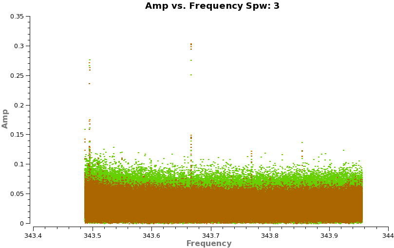
[[Image: | [[Image:Birdies_spw2_X3x1.png|thumb|Phase calibrators (brown and green) and TW Hya (orange) showing both real CO(3-2) emission in TW Hya and weak ''birdie'' spectral features in all three sources for spw=2.]] | ||
With such high spectral resolution data, one often sees occasional "birdies" in the data. These are typically very narrow weak spectral features that are internally generated in the system. Over time as we track down issues the number of birdies should decrease, but you should always check. This is easiest to do by looking at amplitude vs. frequency for sources observed over a long time range (for sensitivity). It is helpful to look at more than one source to verify the nature of the emission. Below we look at both calibrators (brown and green) and TW Hya (orange). If you have enough sensitivity birdies should be seen on all sources, however, be careful not to mistake real line emission for a birdie even on a calibrator - they can be present as we've seen for Titan. | With such high spectral resolution data, one often sees occasional "birdies" in the data. These are typically very narrow weak spectral features that are internally generated in the system. Over time as we track down issues the number of birdies should decrease, but you should always check. This is easiest to do by looking at amplitude vs. frequency for sources observed over a long time range (for sensitivity). It is helpful to look at more than one source to verify the nature of the emission. Below we look at both calibrators (brown and green) and TW Hya (orange). If you have enough sensitivity birdies should be seen on all sources, however, be careful not to mistake real line emission for a birdie even on a calibrator - they can be present as we've seen for Titan. | ||
[[Image: | [[Image:Birdies_spw3_X3x1.png|thumb|Phase calibrators (brown and green) and TW Hya (orange) showing only weak birdie spectral features in spw=3.]] | ||
<source lang="python"> | <source lang="python"> | ||
| Line 403: | Line 406: | ||
Replot in {{plotms}} to check that flagging has been done as anticipated. | Replot in {{plotms}} to check that flagging has been done as anticipated. | ||
==Flag Calibrator Spectral Features== | ==Flag Calibrator Spectral Features== | ||
| Line 465: | Line 417: | ||
<source lang="python"> | <source lang="python"> | ||
# In CASA | # In CASA | ||
plotms(vis=' | basename=["X3c1_wvrtsys","X5d8_wvrtsys","X7ef_wvrtsys"] | ||
for asdm in basename: | |||
plotms(vis=asdm+'.ms',spw='',xaxis='channel',yaxis='amp',field='0,1', | |||
avgtime='1e8',coloraxis='field',iteraxis='spw') | |||
print('When you are done with the graphics window,') | |||
print('quit that window, and') | |||
user_check=raw_input('press enter to continue script\n') | |||
</source> | </source> | ||
| Line 473: | Line 430: | ||
<source lang="python"> | <source lang="python"> | ||
# In CASA | # In CASA | ||
plotms(vis=' | for asdm in basename: | ||
plotms(vis=asdm+'.ms',spw='2:1600~2300',xaxis='frequency',yaxis='amp', | |||
field='0',avgtime='1e8',coloraxis='field') | |||
print('When you are done with the graphics window,') | |||
print('quit that window, and') | |||
user_check=raw_input('press enter to continue script\n') | |||
</source> | </source> | ||
| Line 483: | Line 444: | ||
<source lang="python"> | <source lang="python"> | ||
# In CASA | # In CASA | ||
plotms(vis=' | for asdm in basename: | ||
plotms(vis=asdm+'.ms',spw='2:1600~2300',xaxis='channel',yaxis='amp', | |||
field='0',avgtime='1e8',coloraxis='field') | |||
print('When you are done with the graphics window,') | |||
print('quit that window, and') | |||
user_check=raw_input('press enter to continue script\n') | |||
</source> | </source> | ||
| Line 491: | Line 456: | ||
<source lang="python"> | <source lang="python"> | ||
# In CASA | # In CASA | ||
plotms(vis=' | for asdm in basename: | ||
plotms(vis=asdm+'.ms',spw='',xaxis='channel',yaxis='amp',field='1', | |||
avgtime='1e8',coloraxis='field',iteraxis='spw') | |||
print('When you are done with the graphics window,') | |||
print('quit that window, and') | |||
user_check=raw_input('press enter to continue script\n') | |||
</source> | </source> | ||
| Line 499: | Line 468: | ||
<source lang="python"> | <source lang="python"> | ||
# In CASA | # In CASA | ||
flagmanager(vis=' | for asdm in basename: | ||
flagmanager(vis=asdm+'.ms',mode='save',versionname=asdm+'.before_calspectralflags') | |||
</source> | </source> | ||
| Line 508: | Line 478: | ||
<source lang="python"> | <source lang="python"> | ||
# In CASA | # In CASA | ||
flagdata(vis=' | for asdm in basename: | ||
print "Flagging absorption features in all sources for "+asdm | |||
flagdata(vis=asdm+'.ms', spw=['1:2000~3840','2:1945~1960']) | |||
</source> | </source> | ||
| Line 516: | Line 488: | ||
<source lang="python"> | <source lang="python"> | ||
# In CASA | # In CASA | ||
flagmanager(vis=' | for asdm in basename: | ||
flagmanager(vis=asdm+'.ms',mode='save',versionname=asdm+'.before_emissionflags') | |||
</source> | </source> | ||
<source lang="python"> | <source lang="python"> | ||
# In CASA | # In CASA | ||
flagdata(vis=' | for asdm in basename: | ||
print "Flagging emission for "+asdm | |||
flagdata(vis=asdm+'.ms', | |||
field=['1'], | |||
spw=['3:1000~3000']) | |||
</source> | </source> | ||
| Line 530: | Line 505: | ||
<source lang="python"> | <source lang="python"> | ||
# In CASA | # In CASA | ||
plotms(vis=' | for asdm in basename: | ||
plotms(vis=asdm+'.ms',spw='',xaxis='channel',yaxis='amp',field='0,1', | |||
avgtime='1e8',coloraxis='field',iteraxis='spw') | |||
print('When you are done with the graphics window,') | |||
print('quit that window, and') | |||
user_check=raw_input('press enter to continue script\n') | |||
</source> | </source> | ||
| Line 540: | Line 519: | ||
<source lang="python"> | <source lang="python"> | ||
# In CASA | # In CASA | ||
setjy(vis=' | basename=["X3c1_wvrtsys","X5d8_wvrtsys","X7ef_wvrtsys"] | ||
for asdm in basename: | |||
setjy(vis=asdm+'.ms',field='1', | |||
standard='Butler-JPL-Horizons 2010',scalebychan=F) | |||
</source> | </source> | ||
==Bandpass Calibration== | ==Bandpass Calibration== | ||
[[Image: | [[Image:ThreeScansAmp.png|thumb|Amplitude variation during the three 3C279 scans (from one representative baseline).]] | ||
[[Image: | [[Image:ThreeScansPhase.png|thumb|Phase variation during the three 3C279 scans (from one representative baseline).]] | ||
First we need to check how the amplitude and phase of 3C279 behave as a function of time. | First we need to check how the amplitude and phase of 3C279 behave as a function of time. | ||
| Line 552: | Line 533: | ||
<source lang="python"> | <source lang="python"> | ||
# In CASA | # In CASA | ||
plotms(vis=' | for asdm in basename: | ||
plotms(vis=asdm+'.ms',spw='',xaxis='time',yaxis='amp', | |||
field='0',avgchannel='3840',iteraxis='spw') | |||
print('When you are done with the graphics window,') | |||
print('quit that window, and') | |||
user_check=raw_input('press enter to continue script\n') | |||
</source> | </source> | ||
| Line 560: | Line 545: | ||
<source lang="python"> | <source lang="python"> | ||
# In CASA | # In CASA | ||
plotms(vis=' | for asdm in basename: | ||
plotms(vis=asdm+'.ms',spw='0',xaxis='time',yaxis='phase', | |||
antenna='DV06;!DV04',coloraxis='corr', | |||
field='0',avgchannel='3840',iteraxis='baseline') | |||
print('When you are done with the graphics window,') | |||
print('quit that window, and') | |||
user_check=raw_input('press enter to continue script\n') | |||
</source> | </source> | ||
| Line 569: | Line 558: | ||
<source lang="python"> | <source lang="python"> | ||
# In CASA | # In CASA | ||
gaincal(vis=' | for asdm in basename: | ||
gaincal(vis=asdm+'.ms',caltable=asdm+'.bpphase.gcal', | |||
field='0',spw='0~3:900~1100',refant='DV06', | |||
calmode='p',solint='int',minsnr=2.0,minblperant=4) | |||
</source> | </source> | ||
[[Image:bpphase.X.png|thumb|Phase only solutions for correlation X on the bandpass calibrator 3C279.]] | [[Image:X7ef_wvrtsys.bpphase.X.png|thumb|Phase-only solutions for correlation X on the third scan of bandpass calibrator 3C279.]] | ||
Inspect the phase-only calibration solutions for the bandpass calibrator. Look for any noisy solutions. We do XX and YY separately to reduce confusion in the plot. It will help if you make your plotcal window wide. | Inspect the phase-only calibration solutions for the bandpass calibrator. Look for any noisy solutions. We do XX and YY separately to reduce confusion in the plot. It will help if you make your plotcal window wide. | ||
| Line 580: | Line 570: | ||
<source lang="python"> | <source lang="python"> | ||
# In CASA | # In CASA | ||
plotcal(caltable='bpphase.gcal',xaxis='time',yaxis='phase',spw='',antenna='1~8', | for asdm in basename: | ||
plotcal(caltable=asdm+'.bpphase.gcal',xaxis='time',yaxis='phase',spw='',antenna='1~8', | |||
iteration='antenna',subplot=421,plotrange=[0,0,-180,180], | |||
figfile=asdm+'.bpphase.X.png',poln='X') | |||
print('When you are done with the graphics window,') | |||
print('quit that window, and') | |||
user_check=raw_input('press enter to continue script\n') | |||
</source> | </source> | ||
| Line 589: | Line 583: | ||
<source lang="python"> | <source lang="python"> | ||
# In CASA | # In CASA | ||
plotcal(caltable='bpphase.gcal',xaxis='time',yaxis='phase',spw='',antenna='1~8', | for asdm in basename: | ||
plotcal(caltable=asdm+'.bpphase.gcal',xaxis='time',yaxis='phase',spw='',antenna='1~8', | |||
iteration='antenna',subplot=421,plotrange=[0,0,-180,180], | |||
figfile=asdm+'.bpphase.Y.png',poln='Y') | |||
print('When you are done with the graphics window,') | |||
print('quit that window, and') | |||
user_check=raw_input('press enter to continue script\n') | |||
</source> | </source> | ||
| Line 598: | Line 596: | ||
<source lang="python"> | <source lang="python"> | ||
# In CASA | # In CASA | ||
bandpass(vis=' | for asdm in basename: | ||
bandpass(vis=asdm+'.ms',caltable=asdm+'.bandpass.bcal', | |||
field='0',spw='',combine='',refant='DV06', | |||
solint='inf',solnorm=T,minblperant=4,fillgaps=17, | |||
gaintable=[asdm+'.bpphase.gcal']) | |||
</source> | </source> | ||
You will see some error messages, these are just related to the flagged channels. We set fillgaps=17 to interpolate across the smaller regions of flagged channels (mesospheric features and birdies). | You will see some error messages, these are just related to the flagged channels. We set fillgaps=17 to interpolate across the smaller regions of flagged channels (mesospheric features and birdies). | ||
[[Image: | [[Image:Bandpass.ampspw0.png|thumb|Bandpass amplitude plots.]] | ||
[[Image: | [[Image:Bandpass.phasespw0.png|thumb|Bandpass phase plots.]] | ||
'''A few words about solint and combine:''' | '''A few words about solint and combine:''' | ||
| Line 618: | Line 617: | ||
<source lang="python"> | <source lang="python"> | ||
# In CASA | # In CASA | ||
plotcal(caltable='bandpass.bcal',xaxis='freq',yaxis='amp',antenna='1~8', | for asdm in basename: | ||
plotcal(caltable=asdm+'.bandpass.bcal',xaxis='freq',yaxis='amp',antenna='1~8', | |||
iteration='antenna',subplot=421,spw='0',figfile=asdm+'.bandpass.ampspw0.png') | |||
print('When you are done with the graphics window,') | |||
print('quit that window, and') | |||
user_check=raw_input('press enter to continue script\n') | |||
</source> | </source> | ||
<source lang="python"> | <source lang="python"> | ||
# In CASA | # In CASA | ||
plotcal(caltable='bandpass.bcal',xaxis='freq',yaxis='phase',antenna='1~8', | for asdm in basename: | ||
plotcal(caltable=asdm+'.bandpass.bcal',xaxis='freq',yaxis='phase',antenna='1~8', | |||
iteration='antenna',subplot=421,spw='0',figfile=asdm+'.bandpass.phasespw0.png') | |||
print('When you are done with the graphics window,') | |||
print('quit that window, and') | |||
user_check=raw_input('press enter to continue script\n') | |||
</source> | </source> | ||
| Line 638: | Line 645: | ||
<source lang="python"> | <source lang="python"> | ||
# In CASA | # In CASA | ||
gaincal(vis=' | basename=["X3c1_wvrtsys","X5d8_wvrtsys","X7ef_wvrtsys"] | ||
for asdm in basename: | |||
gaincal(vis=asdm+'.ms',caltable=asdm+'.intphase.gcal', | |||
field='0,1,3,4',spw='0~3:40~3800',refant='DV06', | |||
calmode='p',solint='int',minsnr=2.0,minblperant=4, | |||
gaintable=[asdm+'.bandpass.bcal']) | |||
</source> | </source> | ||
| Line 650: | Line 659: | ||
<source lang="python"> | <source lang="python"> | ||
# In CASA | # In CASA | ||
gaincal(vis=' | for asdm in basename: | ||
gaincal(vis=asdm+'.ms',caltable=asdm+'.scanphase.gcal', | |||
field='0,1,3,4',spw='0~3:40~3800',refant='DV06', | |||
calmode='p',solint='inf',minsnr=2.0,minblperant=4, | |||
gaintable=[asdm+'.bandpass.bcal']) | |||
</source> | </source> | ||
| Line 662: | Line 672: | ||
<source lang="python"> | <source lang="python"> | ||
# In CASA | # In CASA | ||
gaincal(vis=' | for asdm in basename: | ||
gaincal(vis=asdm+'.ms',caltable=asdm+'.amp.gcal', | |||
field='0,1,3,4',spw='0~3:40~3800',refant='DV06', | |||
calmode='ap',solint='inf',minsnr=2.0,minblperant=4, | |||
gaintable=[asdm+'.bandpass.bcal',asdm+'.intphase.gcal']) | |||
</source> | </source> | ||
| Line 671: | Line 682: | ||
We make plots in X and Y separately for clarity. The colors are showing the spectral windows. | We make plots in X and Y separately for clarity. The colors are showing the spectral windows. | ||
[[Image:intphase_X.png|thumb|Phase solutions for every integration time.]] | [[Image:X3c1_wvrtsys.intphase_X.png|thumb|Phase solutions for the X polarization for every integration time of the first dataset.]] | ||
[[Image:scanphase_X.png|thumb|Phase solutions for | [[Image:X3c1_wvrtsys.scanphase_X.png|thumb|Phase solutions for the X polarization for every for every scan of the first dataset.]] | ||
<source lang="python"> | <source lang="python"> | ||
# In CASA | # In CASA | ||
plotcal(caltable='intphase.gcal',xaxis='time',yaxis='phase',antenna='1~8', | for asdm in basename: | ||
plotcal(caltable=asdm+'.intphase.gcal',xaxis='time',yaxis='phase',antenna='1~8', | |||
spw='',field='0,1,3,4',iteration='antenna',subplot=421, | |||
plotrange=[0,0,-180,180],poln='X',figfile=asdm+'.intphase_X.png') | |||
print('When you are done with the graphics window,') | |||
print('quit that window, and') | |||
user_check=raw_input('press enter to continue script\n') | |||
</source> | </source> | ||
<source lang="python"> | <source lang="python"> | ||
# In CASA | # In CASA | ||
plotcal(caltable='intphase.gcal',xaxis='time',yaxis='phase',antenna='1~8', | for asdm in basename: | ||
plotcal(caltable=asdm+'.intphase.gcal',xaxis='time',yaxis='phase',antenna='1~8', | |||
spw='',field='0,1,3,4',iteration='antenna',subplot=421, | |||
plotrange=[0,0,-180,180],poln='Y',figfile=asdm+'.intphase_Y.png') | |||
print('When you are done with the graphics window,') | |||
print('quit that window, and') | |||
user_check=raw_input('press enter to continue script\n') | |||
</source> | </source> | ||
<source lang="python"> | <source lang="python"> | ||
# In CASA | # In CASA | ||
plotcal(caltable='scanphase.gcal',xaxis='time',yaxis='phase',antenna='1~8', | for asdm in basename: | ||
plotcal(caltable=asdm+'.scanphase.gcal',xaxis='time',yaxis='phase',antenna='1~8', | |||
spw='',field='0,1,3,4',iteration='antenna',subplot=421, | |||
plotrange=[0,0,-180,180],poln='X',figfile=asdm+'.scanphase_X.png') | |||
print('When you are done with the graphics window,') | |||
print('quit that window, and') | |||
user_check=raw_input('press enter to continue script\n') | |||
</source> | </source> | ||
<source lang="python"> | <source lang="python"> | ||
# In CASA | # In CASA | ||
plotcal(caltable='scanphase.gcal',xaxis='time',yaxis='phase',antenna='1~8', | for asdm in basename: | ||
plotcal(caltable=asdm+'.scanphase.gcal',xaxis='time',yaxis='phase',antenna='1~8', | |||
spw='',field='0,1,3,4',iteration='antenna',subplot=421, | |||
plotrange=[0,0,-180,180],poln='Y',figfile=asdm+'.scanphase_Y.png') | |||
print('When you are done with the graphics window,') | |||
print('quit that window, and') | |||
user_check=raw_input('press enter to continue script\n') | |||
</source> | </source> | ||
[[Image:amp_phase.png|thumb|Residual phase after applying intphase.gcal for both correlations.]] | [[Image:X3c1_wvrtsys.amp_phase.png|thumb|Residual phase after applying intphase.gcal for both correlations in the first dataset.]] | ||
[[Image:amp_X.png|thumb|Amplitude solutions on a scan interval for correlation X.]] | [[Image:X3c1_wvrtsys.amp_X.png|thumb|Amplitude solutions on a scan interval for correlation X in the first dataset.]] | ||
Since we have taken out the phase as best we can by applying the solint='int' phase-only solution, this plot will give a good idea of the residual phase error. If you see scatter of more than a few degrees here, you should consider going back and looking for more data to flag, particularly bad timeranges etc. | Since we have taken out the phase as best we can by applying the solint='int' phase-only solution, this plot will give a good idea of the residual phase error. If you see scatter of more than a few degrees here, you should consider going back and looking for more data to flag, particularly bad timeranges etc. | ||
| Line 710: | Line 736: | ||
<source lang="python"> | <source lang="python"> | ||
# In CASA | # In CASA | ||
plotcal(caltable='amp.gcal',xaxis='time',yaxis='phase',antenna='1~8', | for asdm in basename: | ||
plotcal(caltable=asdm+'.amp.gcal',xaxis='time',yaxis='phase',antenna='1~8', | |||
spw='',field='0,1,3,4',plotrange=[0,0,-1,1], | |||
iteration='antenna',subplot=421,figfile=asdm+'.amp_phase.png') | |||
print('When you are done with the graphics window,') | |||
print('quit that window, and') | |||
user_check=raw_input('press enter to continue script\n') | |||
</source> | </source> | ||
| Line 719: | Line 749: | ||
<source lang="python"> | <source lang="python"> | ||
# In CASA | # In CASA | ||
plotcal(caltable='amp.gcal',xaxis='time',yaxis='amp',antenna='1~8', | for asdm in basename: | ||
plotcal(caltable=asdm+'.amp.gcal',xaxis='time',yaxis='amp',antenna='1~8', | |||
iteration='antenna',subplot=421,spw='',poln='X', | |||
plotrange=[0,0,0.0,0.3],figfile=asdm+'.amp_X.png') | |||
print('When you are done with the graphics window,') | |||
print('quit that window, and') | |||
user_check=raw_input('press enter to continue script\n') | |||
</source> | </source> | ||
<source lang="python"> | <source lang="python"> | ||
# In CASA | # In CASA | ||
plotcal(caltable='amp.gcal',xaxis='time',yaxis='amp',antenna='1~8', | for asdm in basename: | ||
plotcal(caltable=asdm+'.amp.gcal',xaxis='time',yaxis='amp',antenna='1~8', | |||
iteration='antenna',subplot=421,spw='',poln='Y', | |||
plotrange=[0,0,0.0,0.3],figfile=asdm+'.amp_Y.png') | |||
print('When you are done with the graphics window,') | |||
print('quit that window, and') | |||
user_check=raw_input('press enter to continue script\n') | |||
</source> | </source> | ||
==Flux Calibration== | |||
Next we use the flux calibrator (whose flux density was set in {{setjy}} above) to derive the flux of the other calibrators. Note that the flux table REPLACES the amp.gcal in terms of future application of the calibration to the data, i.e. the flux table contains both the amp.gcal and flux scaling. Unlike the gain calibration steps, this is not an incremental table. | Next we use the flux calibrator (whose flux density was set in {{setjy}} above) to derive the flux of the other calibrators. Note that the flux table REPLACES the amp.gcal in terms of future application of the calibration to the data, i.e. the flux table contains both the amp.gcal and flux scaling. Unlike the gain calibration steps, this is not an incremental table. | ||
| Line 735: | Line 775: | ||
<source lang="python"> | <source lang="python"> | ||
# In CASA | # In CASA | ||
fluxscale(vis=' | for asdm in basename: | ||
fluxscale(vis=asdm+'.ms',caltable=asdm+'.amp.gcal', | |||
fluxtable=asdm+'.flux.cal',reference='1',refspwmap=[0,1,3,3]) | |||
</source> | </source> | ||
| Line 759: | Line 800: | ||
</pre> | </pre> | ||
[[Image:flux_X.png|thumb|Absolute flux calibration solutions for correlation X]] | [[Image:X3c1_wvrtsys.flux_X.png|thumb|Absolute flux calibration solutions for correlation X for the first dataset.]] | ||
Now look at the flux solutions. | Now look at the flux solutions. | ||
| Line 765: | Line 806: | ||
<source lang="python"> | <source lang="python"> | ||
# In CASA | # In CASA | ||
plotcal(caltable='flux.cal',xaxis='time',yaxis='amp',antenna='1~8', | for asdm in basename: | ||
plotcal(caltable=asdm+'.flux.cal',xaxis='time',yaxis='amp',antenna='1~8', | |||
iteration='antenna',subplot=421,spw='',poln='X', | |||
plotrange=[0,0,0.0,0.3],figfile=asdm+'.flux_X.png') | |||
print('When you are done with the graphics window,') | |||
print('quit that window, and') | |||
user_check=raw_input('press enter to continue script\n') | |||
</source> | </source> | ||
<source lang="python"> | <source lang="python"> | ||
# In CASA | # In CASA | ||
plotcal(caltable='flux.cal',xaxis='time',yaxis='amp',antenna='1~8', | for asdm in basename: | ||
plotcal(caltable=asdm+'.flux.cal',xaxis='time',yaxis='amp',antenna='1~8', | |||
iteration='antenna',subplot=421,spw='',poln='Y', | |||
plotrange=[0,0,0.0,0.3],figfile=asdm+'.flux_Y.png') | |||
print('When you are done with the graphics window,') | |||
print('quit that window, and') | |||
user_check=raw_input('press enter to continue script\n') | |||
</source> | </source> | ||
==Apply Calibration and Inspect== | ==Apply Calibration and Inspect== | ||
Now we can use the {{flagmanager}} to restore the spectral flagging we did on the | Now we can use the {{flagmanager}} if we want to restore any of the spectral flagging we did prior to bandpass calibration. | ||
In this case, we choose to restore the flags of the emission lines on Titan, because we are interested in seeing how | |||
strong they are compared to the continuum. However, we leave the strong ozone line and mesospheric CO line flagged on all | |||
sources, because we want to get the most accurate continuum flux density for the science target. | |||
<source lang="python"> | <source lang="python"> | ||
# In CASA | # In CASA | ||
flagmanager(vis=' | basename=["X3c1_wvrtsys","X5d8_wvrtsys","X7ef_wvrtsys"] | ||
for asdm in basename: | |||
flagmanager(vis=asdm+'.ms',mode='restore',versionname=asdm+'.before_emissionflags') | |||
</source> | </source> | ||
| Line 792: | Line 846: | ||
<source lang="python"> | <source lang="python"> | ||
# In CASA | # In CASA | ||
applycal(vis=' | for asdm in basename: | ||
applycal(vis=asdm+'.ms',field='0', | |||
gaintable=[asdm+'.bandpass.bcal',asdm+'.intphase.gcal',asdm+'.flux.cal'], | |||
interp=['nearest','nearest','nearest'], | |||
gainfield=['0','0','0'],flagbackup=T) | |||
</source> | </source> | ||
| Line 802: | Line 857: | ||
<source lang="python"> | <source lang="python"> | ||
# In CASA | # In CASA | ||
applycal(vis=' | for asdm in basename: | ||
applycal(vis=asdm+'.ms',field='1', | |||
gaintable=[asdm+'.bandpass.bcal',asdm+'.intphase.gcal',asdm+'.flux.cal'], | |||
interp=['nearest','nearest','nearest'], | |||
gainfield=['0','1','1'], flagbackup=T, calwt=F) | |||
</source> | </source> | ||
For the secondary phase calibrator, we apply the phase and flux solutions from the primary phase calibrator. This will allow us to | For the secondary phase calibrator, we apply the phase and flux solutions from the primary phase calibrator. This will allow us to independently assess how well the phase transfer to the science target (TW Hya) has worked: | ||
<source lang="python"> | <source lang="python"> | ||
# In CASA | # In CASA | ||
applycal(vis=' | for asdm in basename: | ||
applycal(vis=asdm+'.ms',field='3', | |||
gaintable=[asdm+'.bandpass.bcal',asdm+'.scanphase.gcal',asdm+'.flux.cal'], | |||
interp=['nearest','linear','linear'], | |||
gainfield=['0','4','4'], flagbackup=T, calwt=F) | |||
</source> | </source> | ||
| Line 822: | Line 879: | ||
<source lang="python"> | <source lang="python"> | ||
# In CASA | # In CASA | ||
applycal(vis=' | for asdm in basename: | ||
applycal(vis=asdm+'.ms',field='4', | |||
gaintable=[asdm+'.bandpass.bcal',asdm+'.intphase.gcal',asdm+'.flux.cal'], | |||
interp=['nearest','nearest','nearest'], | |||
gainfield=['0','4','4'], flagbackup=T, calwt=F) | |||
</source> | </source> | ||
| Line 832: | Line 890: | ||
<source lang="python"> | <source lang="python"> | ||
# In CASA | # In CASA | ||
applycal(vis=' | for asdm in basename: | ||
applycal(vis=asdm+'.ms',field='2', | |||
interp=['nearest','linear','linear'], | |||
gaintable=[asdm+'.bandpass.bcal',asdm+'.scanphase.gcal',asdm+'.flux.cal'], | |||
gainfield=['0','3,4','3,4'], flagbackup=T, calwt=F) | |||
</source> | </source> | ||
Now we can check the results of applying the calibration solutions. | Now we can check the results of applying the calibration solutions. | ||
[[Image: | [[Image:Corrected_vs_time_1_3.3.png|thumb|All the calibrated data from the first dataset (amplitude vs. time).]] | ||
<source lang="python"> | <source lang="python"> | ||
# In CASA | # In CASA | ||
plotms(vis=' | for asdm in basename: | ||
plotms(vis=asdm+'.ms',spw='',xaxis='time',yaxis='amp',field='',avgchannel='3840', | |||
coloraxis='field',iteraxis='spw',ydatacolumn='corrected') | |||
print('When you are done with the graphics window,') | |||
print('quit that window, and') | |||
user_check=raw_input('press enter to continue script\n') | |||
</source> | </source> | ||
In amplitude, it looks good but there are some noisy points toward the end of the first scheduling block, but it mostly only affects the secondary phase calibrator (green). In phase, we expect all the points to cluster about zero. The large scatter in phase on the secondary phase calibrator is readily apparent: | |||
[[Image:Corrected_phase_vs_time_1_3.3.png|thumb|The calibrated data on the calibrators from the first dataset (phase vs. time).]] | |||
<source lang="python"> | <source lang="python"> | ||
# In CASA | # In CASA | ||
for asdm in basename: | |||
plotms(vis=asdm+'.ms',spw='',xaxis='time',yaxis='phase',field='0,1,3,4',avgchannel='3840', | |||
coloraxis='field',iteraxis='spw',ydatacolumn='corrected') | |||
print('When you are done with the graphics window,') | |||
print('quit that window, and') | |||
user_check=raw_input('press enter to continue script\n') | |||
</source> | </source> | ||
Let's check whether the situation improves when we apply this calibrator's solutions to itself rather than transferring the solutions from the primary phase calibrator (which is 17 degrees away, and observed at a different time). | |||
<source lang="python"> | <source lang="python"> | ||
# In CASA | # In CASA | ||
for asdm in basename: | |||
applycal(vis=asdm+'.ms',field='3', | |||
gaintable=[asdm+'.bandpass.bcal',asdm+'.intphase.gcal',asdm+'.flux.cal'], | |||
interp=['nearest','nearest','nearest'], | |||
gainfield=['0','3','3'], flagbackup=T, calwt=F) | |||
</source> | </source> | ||
[[Image:Corrected_vs_time_1_field3.png|thumb|The calibrated data from the first dataset (amplitude vs. time), but now field 3 (the secondary phase calibrator) has been calibrated with itself.]] | |||
<source lang="python"> | |||
# In CASA | |||
for asdm in basename: | |||
plotms(vis=asdm+'.ms',spw='',xaxis='time',yaxis='amp',field='',avgchannel='3840', | |||
coloraxis='field',iteraxis='spw',ydatacolumn='corrected') | |||
print('When you are done with the graphics window,') | |||
print('quit that window, and') | |||
user_check=raw_input('press enter to continue script\n') | |||
</source> | |||
[[Image: | [[Image:Corrected_phase_vs_time_1_field3.png|thumb|The calibrated data on the calibrators for the first dataset (phase vs. time), but now field 3 (the secondary phase calibrator) has been calibrated with itself.]] | ||
<source lang="python"> | <source lang="python"> | ||
# In CASA | # In CASA | ||
plotms(vis=' | for asdm in basename: | ||
plotms(vis=asdm+'.ms',spw='',xaxis='time',yaxis='phase',field='0,1,3,4',avgchannel='3840', | |||
coloraxis='field',iteraxis='spw',ydatacolumn='corrected') | |||
print('When you are done with the graphics window,') | |||
print('quit that window, and') | |||
user_check=raw_input('press enter to continue script\n') | |||
</source> | </source> | ||
[[Image: | Indeed, the secondary calibrator looks better now in amplitude and phase. This is an indication that the calibration transfer is not working well in this timerange. Because the effect is not catastrophic and we know we can self-calibrate on TW Hya later, we will let this go for now. Or if you want you can delve deeper into the data and try to solve the mystery... In any case, so that we can later check the effect of correcting the secondary phase calibrator with the primary phase calibrator, we will re-issue the original {{applycal}} so that it is this calibration that our subsequent {{split}} will use. | ||
<source lang="python"> | |||
# In CASA | |||
for asdm in basename: | |||
applycal(vis=asdm+'.ms',field='3', | |||
gaintable=[asdm+'.bandpass.bcal', asdm+'.scanphase.gcal', asdm+'.flux.cal'], | |||
interp=['nearest','linear','linear'], | |||
gainfield=['0','4','4'], flagbackup=T, calwt=F) | |||
</source> | |||
Let's examine the spectral calibration now. First, 3C279 and Titan: | |||
[[Image:X3c1_spw2_corrected.png|thumb|Spectral UV-plots of 3C279 and Titan of spw=2 for the first dataset.]] | |||
<source lang="python"> | <source lang="python"> | ||
# In CASA | # In CASA | ||
plotms(vis=' | for asdm in basename: | ||
plotms(vis=asdm+'.ms',spw='',xaxis='frequency',yaxis='amp',field='0,1', | |||
avgtime='1e8',avgscan=T,coloraxis='field',ydatacolumn='corrected', | |||
iteraxis='spw',xselfscale=T) | |||
print('When you are done with the graphics window,') | |||
print('quit that window, and') | |||
user_check=raw_input('press enter to continue script\n') | |||
</source> | </source> | ||
| Line 895: | Line 994: | ||
<source lang="python"> | <source lang="python"> | ||
# In CASA | # In CASA | ||
plotms(vis=' | for asdm in basename: | ||
plotms(vis=asdm+'.ms',spw='',xaxis='frequency',yaxis='amp',field='3,4', | |||
avgtime='1e8',avgscan=T,coloraxis='field',ydatacolumn='corrected', | |||
iteraxis='spw',xselfscale=T) | |||
print('When you are done with the graphics window,') | |||
print('quit that window, and') | |||
user_check=raw_input('press enter to continue script\n') | |||
</source> | </source> | ||
| Line 906: | Line 1,009: | ||
<source lang="python"> | <source lang="python"> | ||
# In CASA | # In CASA | ||
plotms(vis=' | for asdm in basename: | ||
plotms(vis=asdm+'.ms',spw='',xaxis='frequency',yaxis='amp',field='2', | |||
avgtime='1e8',avgscan=T,coloraxis='field',ydatacolumn='corrected', | |||
iteraxis='spw',xselfscale=T) | |||
print('When you are done with the graphics window,') | |||
print('quit that window, and') | |||
user_check=raw_input('press enter to continue script\n') | |||
</source> | </source> | ||
[[Image: | [[Image:X3c1_CO3_2_uvplot.png|thumb|UV-Plot of the TW Hya CO(3-2) emission from the first dataset.]] | ||
[[Image: | [[Image:X3c1_HCO+_uvplot.png|thumb|UV-Plot of the TW Hya HCO+(4-3) emission from the first dataset.]] | ||
We see HCO+(4-3) in spw=0 and CO(3-2) in spw=2 as expected. Because the shape of the | We see HCO+(4-3) in spw=0 and CO(3-2) in spw=2 as expected. Because the shape of the | ||
| Line 923: | Line 1,030: | ||
<source lang="python"> | <source lang="python"> | ||
# In CASA | # In CASA | ||
plotms(vis=' | for asdm in basename: | ||
plotms(vis=asdm+'.ms',spw='2',xaxis='velocity',yaxis='amp',field='2', | |||
avgtime='1e8',avgscan=T,transform=T,freqframe='LSRK',restfreq='345.79599GHz', | |||
plotrange=[-10,15,0,0],coloraxis='spw') | |||
print('When you are done with the graphics window,') | |||
print('quit that window, and') | |||
user_check=raw_input('press enter to continue script\n') | |||
</source> | </source> | ||
<source lang="python"> | <source lang="python"> | ||
# In CASA | # In CASA | ||
plotms(vis=' | for asdm in basename: | ||
plotms(vis=asdm+'.ms',spw='0',xaxis='velocity',yaxis='amp',field='2', | |||
avgtime='1e8',avgscan=T,transform=T,freqframe='LSRK',restfreq='356.7342GHz', | |||
plotrange=[-10,15,0,0],coloraxis='spw') | |||
print('When you are done with the graphics window,') | |||
print('quit that window, and') | |||
user_check=raw_input('press enter to continue script\n') | |||
</source> | </source> | ||
Both lines show up at the expected velocity. | Both lines show up at the expected velocity. | ||
==Concatenate the Data== | |||
Here we will concatenate the three calibrated datasets prior to imaging. | |||
<source lang="python"> | |||
# In CASA | |||
splitdata=['X3c1_wvrtsys.ms','X5d8_wvrtsys.ms','X7ef_wvrtsys.ms'] | |||
os.system('rm -rf Band7multi_april22.ms') | |||
concat(vis=splitdata,concatvis='Band7multi_april22.ms') | |||
</source> | |||
If you like you can run listobs on new combined dataset: | |||
<source lang="python"> | |||
# In CASA | |||
listobs(vis='Band7multi_april22.ms',verbose=F) | |||
</source> | |||
You can also examine the spectral uv plots for the combined dataset to see the improvement in S/N: | |||
[[Image:All_spw2_corrected.png|thumb|Spectral UV-plots of 3C279 and Titan of spw=2 for the combined datasets.]] | |||
<source lang="python"> | |||
# In CASA | |||
for asdm in basename: | |||
plotms(vis='Band7multi_april22.ms',spw='',xaxis='frequency',yaxis='amp',field='0,1', | |||
avgtime='1e8',avgscan=T,coloraxis='field',ydatacolumn='corrected', | |||
iteraxis='spw',xselfscale=T) | |||
print('When you are done with the graphics window,') | |||
print('quit that window, and') | |||
user_check=raw_input('press enter to continue script\n') | |||
</source> | |||
...and the CO line profile for the combined dataset: | |||
[[Image:All_CO3_2_uvplot.png|thumb|UV-Plot of the TW Hya CO(3-2) emission from the combined datasets.]] | |||
<source lang="python"> | |||
# In CASA | |||
for asdm in basename: | |||
plotms(vis='Band7multi_april22.ms',spw='2',xaxis='velocity',yaxis='amp',field='2', | |||
avgtime='1e8',avgscan=T,transform=T,freqframe='LSRK',restfreq='345.79599GHz', | |||
plotrange=[-10,15,0,0],coloraxis='spw') | |||
print('When you are done with the graphics window,') | |||
print('quit that window, and') | |||
user_check=raw_input('press enter to continue script\n') | |||
</source> | |||
==Fix Titan's Coordinates== | |||
'''Note that in the near future this step will be unnecessary.''' | |||
It is temporarily necessary to correct the positions of ephemeris objects observed by ALMA, as they are currently erroneously written to the data with coordinates of 00:00:00.0000 +00.00.00.0000 J2000 (see {{listobs}} output in [[TWHydraBand7_Calibration#Observing_Log_and_Priors]]). For this data we need to correct Titan which we observed as the absolute flux calibrator. It is important to apply the fix after concatenation of the data, or Titan will be at slightly different positions in all three datasets. | |||
If you are running casa revision r15777 or newer, fixplanets() is already defined as a task. However, if you are using an older revision, then you must first initialize this script with this command: | |||
execfile(casadef.python_library_directory+'/recipes/fixplanets.py') | |||
Now fix the position of Titan. This step takes a while because the model and corrected scratch columns must be created for the new dataset first (see logger message). | |||
<source lang="python"> | |||
# In CASA | |||
fixplanets(vis='Band7multi_april22.ms', field='Titan', fixuvw=True) | |||
</source> | |||
Check the header information again to see that the information for Titan has changed. | |||
<source lang="python"> | |||
# In CASA | |||
listobs(vis='Band7multi_april22.ms',verbose=F) | |||
</source> | |||
<pre style="background-color: #fffacd;"> | |||
ID Code Name RA Decl Epoch SrcId | |||
0 none 3c279 12:56:11.1666 -05.47.21.5247 J2000 0 | |||
1 none Titan 12:49:26.5120 -02.22.10.8190 J2000 1 | |||
2 none TW Hya 11:01:51.9063 -34.42.17.0212 J2000 2 | |||
3 none J1147-382=Q* 11:47:01.3815 -38.12.11.1179 J2000 3 | |||
4 none J1037-295=Q* 10:37:16.0899 -29.34.02.9888 J2000 4 | |||
</pre> | |||
==Split Calibrated Data== | ==Split Calibrated Data== | ||
| Line 960: | Line 1,156: | ||
split(vis='Band7multi_april22.ms',outputvis='J1147_corrected.ms', | split(vis='Band7multi_april22.ms',outputvis='J1147_corrected.ms', | ||
datacolumn='corrected',spw='',field='3') | datacolumn='corrected',spw='',field='3') | ||
</source> | </source> | ||
| Line 983: | Line 1,169: | ||
os.system('rm -rf Titan_cont.ms') | os.system('rm -rf Titan_cont.ms') | ||
split(vis='Band7multi_april22.ms',outputvis='Titan_cont.ms', | split(vis='Band7multi_april22.ms',outputvis='Titan_cont.ms', | ||
datacolumn='corrected',spw='0',field='1') | |||
</source> | </source> | ||
| Line 990: | Line 1,176: | ||
os.system('rm -rf Titan_CO3_2.ms') | os.system('rm -rf Titan_CO3_2.ms') | ||
split(vis='Band7multi_april22.ms',outputvis='Titan_CO3_2.ms', | split(vis='Band7multi_april22.ms',outputvis='Titan_CO3_2.ms', | ||
datacolumn='corrected',spw='2',field='1') | |||
</source> | </source> | ||
| Line 997: | Line 1,183: | ||
os.system('rm -rf Titan_unknown.ms') | os.system('rm -rf Titan_unknown.ms') | ||
split(vis='Band7multi_april22.ms',outputvis='Titan_unknown.ms', | split(vis='Band7multi_april22.ms',outputvis='Titan_unknown.ms', | ||
datacolumn='corrected',spw='3',field='1') | |||
</source> | </source> | ||
Latest revision as of 20:45, 23 April 2012
- This script assumes that you have downloaded TWHYA_BAND7_UnCalibratedMSAndTablesForReduction.tgz from TWHydraBand7#Getting_the_Data
- Details of the ALMA data are provided at TWHydraBand7
- Older version of the calibration part of the tutorial can be found at: TWHydraBand7_Old_for_CASA_3.3
Unpack the Data
Once you have downloaded TWHYA_BAND7_UnCalibratedMSAndTablesForReduction.tgz, in a terminal unpack it with
>tar -zxvf TWHYA_BAND7_UnCalibratedMSAndTablesForReduction.tgz
Please be aware that you will need about 100 GB of free space to do the data reduction. It is a good idea to check that now before you begin. Some of the plots described here require 9 GB of RAM; as little as 4 GB may be sufficient if additional data averaging is used when the plots are generated. When you are satisfied with the available drive space and memory on your machine:
>cd TWHYA_BAND7_UnCalibratedMSAndTablesForReduction
Then start CASA.
>casapy
Observing Log and Priors
Below is some information that may not be obvious from the data
Like at most telescopes, the ALMA operators and astronomers at the site log any significant issues
that were noticed from the online system during the observation. For these Band 7 observations of
TW Hya on April 22, 2011, the only issue of note was that antenna DV04 could not observe at Band 7
and will need to be flagged.
First let's examine the basic properties of the data using listobs. Among other information we will be able to deduce what the source IDs are and what each source was used for:
3c279 is the bandpass calibrator (field id=0)
Titan is the absolute flux calibrator (field id=1)
J1147-382 is the secondary phase calibrator (field id=3)
J1037-295 is the primary phase calibrator field id=4)
# In CASA
data=['X3c1.ms','X5d8.ms','X7ef.ms']
for vis in data:
  listobs(vis=vis,verbose=T)
Below we copy select parts of the listobs output reported in the CASA logger for reference.
X3c1.ms:
Data records: 278352       Total integration time = 6109.06 seconds
   Observed from   22-Apr-2011/00:01:52.9   to   22-Apr-2011/01:43:42.0 (UTC)

X5d8.ms:
Data records: 278406       Total integration time = 5995.01 seconds
   Observed from   22-Apr-2011/01:48:05.8   to   22-Apr-2011/03:28:00.8 (UTC)

X7ef.ms:
Data records: 255717       Total integration time = 5407.49 seconds
   Observed from   22-Apr-2011/03:30:39.7   to   22-Apr-2011/05:00:47.2 (UTC)

  ID   Code Name         RA            Decl           Epoch   SrcId
  0    none 3c279        12:56:11.1666 -05.47.21.5247 J2000   0
  1    none Titan        00:00:00.0000 +00.00.00.0000 J2000   1
  2    none TW Hya       11:01:51.8450 -34.42.17.1609 J2000   2
  3    none J1147-382=Q* 11:47:01.3815 -38.12.11.1179 J2000   3
  4    none J1037-295=Q* 10:37:16.0899 -29.34.02.9888 J2000   4

  SpwID  Chans Frame Ch1(MHz)    ChanWid(kHz)TotBW(kHz)  Ref(MHz)    Corrs
  0           4 TOPO  184550      1500000     7500000     183300      I
  1         128 TOPO  355740.062  15625       2000000     355732.25   XX  YY
  2           1 TOPO  356716.625  1796875     1796875     355732.25   XX  YY
  3         128 TOPO  356507.813  15625       2000000     356500      XX  YY
  4           1 TOPO  357484.375  1796875     1796875     356500      XX  YY
  5         128 TOPO  346792.187  15625       2000000     346800      XX  YY
  6           1 TOPO  345784.375  1796875     1796875     346800      XX  YY
  7         128 TOPO  345182.438  15625       2000000     345190.25   XX  YY
  8           1 TOPO  344174.625  1796875     1796875     345190.25   XX  YY
  9         128 TOPO  344386.763  15625       2000000     344394.575  XX  YY
  10          1 TOPO  343378.95   1796875     1796875     344394.575  XX  YY
  11        128 TOPO  346324.263  15625       2000000     346332.075  XX  YY
  12          1 TOPO  345316.45   1796875     1796875     346332.075  XX  YY
  13        128 TOPO  354402.388  15625       2000000     354394.575  XX  YY
  14          1 TOPO  355378.95   1796875     1796875     354394.575  XX  YY
  15        128 TOPO  356402.388  15625       2000000     356394.575  XX  YY
  16          1 TOPO  357378.95   1796875     1796875     356394.575  XX  YY
  17       3840 TOPO  356497.936  122.070312  468750      355732.25   XX  YY
  18          1 TOPO  356732.189  468750      468750      355732.25   XX  YY
  19       3840 TOPO  357734.314  122.070312  468750      356500      XX  YY
  20          1 TOPO  357499.939  468750      468750      356500      XX  YY
  21       3840 TOPO  346034.314  122.070312  468750      346800      XX  YY
  22          1 TOPO  345799.939  468750      468750      346800      XX  YY
  23       3840 TOPO  343955.936  122.070312  468750      345190.25   XX  YY
  24          1 TOPO  344190.189  468750      468750      345190.25   XX  YY

   ID=   0-3: 'DV04'='J505', 'DV06'='T704', 'DV07'='J510', 'DV08'='T703',
   ID=   4-7: 'DV09'='N602', 'DV10'='N606', 'PM01'='T702', 'PM02'='T701',
   ID=   8-8: 'PM03'='J504'
Things to Notice from above:
- There are three different data sets acquired close together in time. We will calibrate each dataset independently and then combine the calibrated data prior to imaging.
- Titan appears to have a position of 0,0. We will fix this later in the tutorial (it is a temporary data capture issue in the ALMA system, Titan was properly tracked during the observation).
- There are a lot of spectral windows! Don't be alarmed. In ALMA data,
- spw=0 is always reserved for the water vapor radiometry data.
- spw=9, 11, 13, 15 are the wideband (TDM) correlator mode with 128 channels per spw default settings for doing pointing and this is all they are used for in these data
- currently Tsys data can only be taken in the wide (TDM) correlator mode with 128 channels per spw, these correspond to spws=1, 3, 5, 7 above. The frequencies of these TDM spw were carefully chosen so the the narrowband FDM spws fall within them.
- The 0.5 GHz, high spectral resolution spws that contain all the real source data (science target and calibrators) are 17, 19, 21, and 23
- For quicklook purposes, the ALMA online system produces a channel averaged spw for each channelized spw, these correspond to spw=2,4,6,8,10,12,14,16,18,20,22,24 and shouldn't be used for anything in post-processing as bandpass calibration etc has not been applied.
Next scroll up in the logger itself after making your logger window as wide as possible (and optionally reducing the font size). In the portion of the listobs that shows the timerange, the final column gives the scan intent. It is important to have a look at this because you can flag and do other operations in CASA using the scan intent as a selection option. Also these intents will be used in the future for pipeline processing. You will usually want to use them to flag the CALIBRATE_POINTING* and CALIBRATE_ATMOS* (the latter correspond to the hot and cold load measurements used to calculate Tsys) data. This is essential for science or calibration data taken only in TDM (wide bandwidth) mode, i.e. the same mode that the pointing and Tsys data are taken in. For the current data however, that calibration data is in different spws from the useful FDM (narrow bandwidth) data, so we'll separate them by splitting them off below.
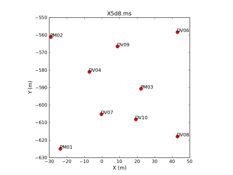
Before we move on, its also nice to get an idea where the antennas are with respect to each other. We can use plotants to plot their positions.
# In CASA
plotants(vis='X5d8.ms',figfile='plot_ants.png')
Examine Tsys and WVR Tables, Apply, and Split
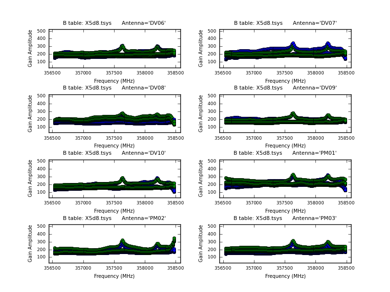
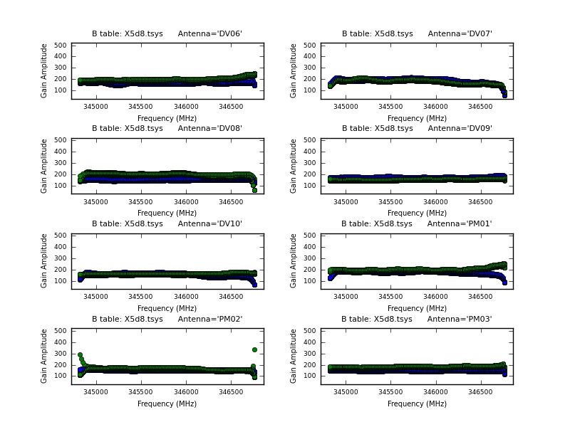
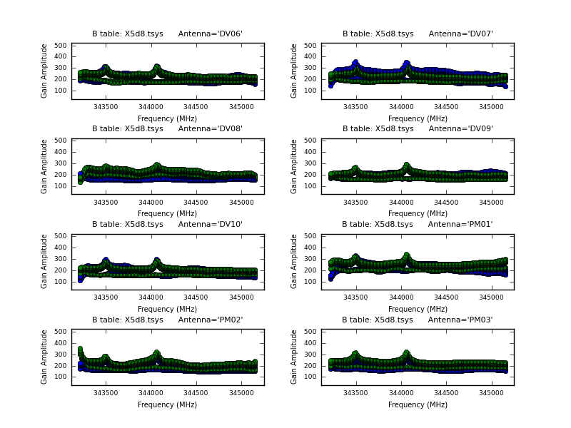
A number of tables were included in the TWHYA_BAND7_UnCalibratedMSAndTablesForReduction directory, including ones of the form *.tsys, *.tsys.fdm, and wvr*cal. The *.tsys tables contain the Tsys values derived from the TDM (wide bandwidth) correlator mode data. They were used to derive Tsys for their corresponding FDM (narrow bandwidth) spws: *.tsys.fdm. The wvr*cal contain the phase corrections derived from the Water Vapor Radiometers. These tables have been provided to you because they are currently generated from scripts rather than inside CASA (for Early Science, these tables will either be pre-applied or supplied with the data).
Below we show plots of the Tsys as a function of frequency plots for the four TDM (broadband) spectral windows for one of the three data sets (X3c1.ms), you can find plots for all the spw, TDM and FDM modes in the directory Tsys_plots/ within the TWHYA_BAND7_RawDataAndTablesForReduction directory.
-
Tsys for the X5d8.ms data, spw=1.
-
Tsys for the X5d8.ms data, spw=3.
-
Tsys for the X5d8.ms data, spw=5.
-
Tsys for the X5d8.ms data, spw=7.
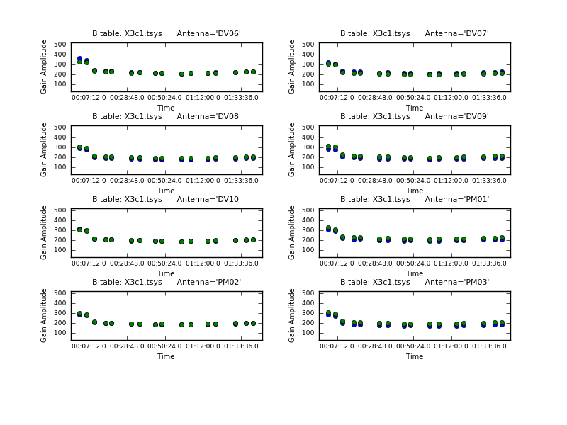
Next we show the Tsys as a function of time for all three datasets.
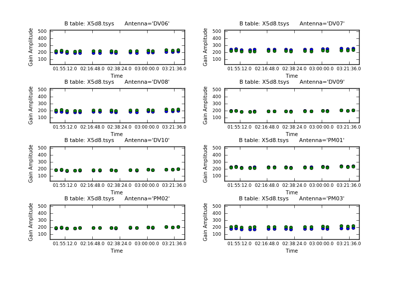
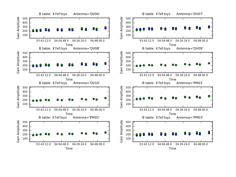
-
Tsys vs Time for the X3c1.ms data.
-
Tsys vs Time for the X5d8.ms data.
-
Tsys vs Time for the X73f.ms data.
It is very important that Tsys measurements taken as close in time and elevation as possible to a particular source are applied. To save time, Tsys measurements are sometimes skipped, so the first step is to establish which sources have their own Tsys measurements and which may not. To do this we will make a plot of X3c1.tsys for each source; if the source has Tsys measurements you will see them (the two polarizations are different colors). We select only one channel to speed plotting.
# In CASA
plotcal(caltable='X3c1.tsys',xaxis='time',yaxis='amp',field='0',antenna='1~8',
        iteration='antenna',subplot=421,poln='',spw='1:50~50')
# In CASA
plotcal(caltable='X3c1.tsys',xaxis='time',yaxis='amp',field='1',antenna='1~8',
        iteration='antenna',subplot=421,poln='',spw='1:50~50')
# In CASA
plotcal(caltable='X3c1.tsys',xaxis='time',yaxis='amp',field='2',antenna='1~8',
        iteration='antenna',subplot=421,poln='',spw='1:50~50')
# In CASA
plotcal(caltable='X3c1.tsys',xaxis='time',yaxis='amp',field='3',antenna='1~8',
        iteration='antenna',subplot=421,poln='',spw='1:50~50')
For this one (field 3) you will get a message like:
2011-05-24 19:51:55 SEVERE Exception Reported: Combined selection selects nothing.
*** Error *** Combined selection selects nothing.
Indicating that there are no Tsys measurements for this source.
# In CASA
plotcal(caltable='X3c1.tsys',xaxis='time',yaxis='amp',field='4',antenna='1~8',
        iteration='antenna',subplot=421,poln='',spw='1:50~50')
So except for Field 3 (the secondary phase calibrator), the other sources including TW Hya itself have their own Tsys measurements. Since the secondary phase calibrator is close on the sky to the primary phase calibrator and observed near in time, we will transfer the Tsys from the primary to the secondary phase calibrator. For sources with Tsys measurements, use the field and gainfield parameters of applycal to apply solutions only to themselves. While applying Tsys, we will also apply the wvr calibration tables; wvr data is usually always present for all sources.
Below we set some definitions so we can loop over the correct parameters.
# In CASA
data=['X3c1.ms','X5d8.ms','X7ef.ms']
fdm='17,19,21,23'
sources=['0','1','2','4']
nocal='3'  # This source had no Tsys measurements associated with it
# In CASA
for vis in data:
  for field in sources:
    applycal(vis=vis,spw=fdm,field=field,gainfield=field,
        gaintable=['%s.tsys.fdm'%(vis.split('.')[0]),'wvr_%s.cal'%(vis.split('.')[0])],
        interp=['nearest','nearest'],flagbackup=F)
For sources without Tsys (i.e. field=3), couple them with best source with Tsys (i.e. field=4).
# In CASA
for vis in data:
  applycal(vis=vis,spw=fdm,field=nocal,
        gaintable=['%s.tsys.fdm'%(vis.split('.')[0]),'wvr_%s.cal'%(vis.split('.')[0])],
        gainfield=['4',nocal],interp=['nearest','nearest'],flagbackup=F)
Check Tsys application with plotms. First we make plots with ydatacolumn='data' to look at the raw data. For simplicity we'll just look at the two strongest sources 3C279 and Titan.
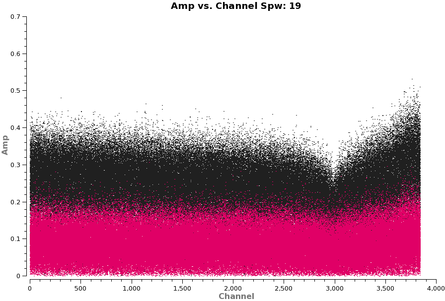
# In CASA
plotms(vis='X5d8.ms',spw='17,19,21,23',xaxis='frequency',yaxis='amp',field='0,1',
       antenna='*&*',avgtime='1e8',avgscan=T,coloraxis='field',iteraxis='spw',
       xselfscale=T,ydatacolumn='data')
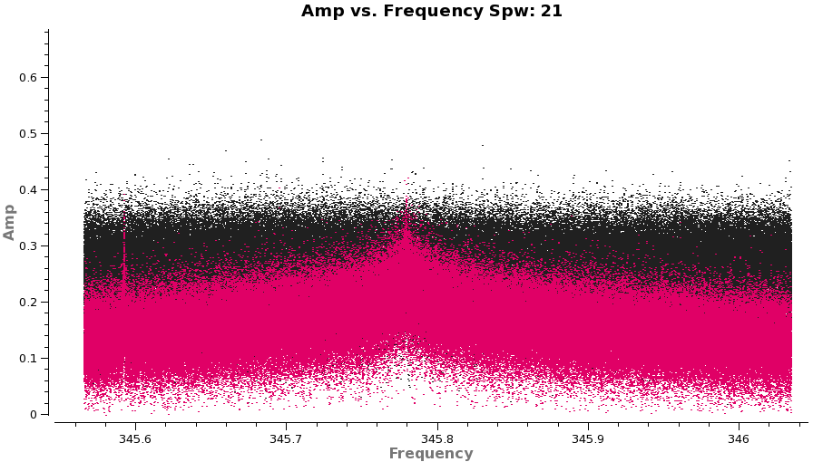
Note: the antenna='*&*' is specifying that we only want to see the cross-correlation data (i.e. not the autocorrelations).
Use the green arrows on the plotms display to cycle through the 4 FDM spws.
Now change Data Column to corrected on the "Axes" tab (this is the same as ydatacolumn in the task) and hit plot button on the gui. Flip through again.
Things to notice:
- The amplitude scale has changed due to application of Tsys
- spw=17 is clean and flat
- spw=19 shows a strong dip around channel 3000 -- this is an atmospheric ozone absorption feature at 357.6 GHz. In the future, high spectral resolution Tsys measurements may help to remove the shape of the absorption, but until then we will need to flag this part of the spectrum.
- spw=21 Titan shows both a narrow and a broad spectral feature. The broad feature is CO(3-2) and it completely fills the 0.5 GHz band so there are no line-free channels! Titan must be handled carefully when it is used as a calibrator because it contains strong line emission. Indeed, we will not be able to use the absolute flux transfer from this spw for other targets. When possible Titan should be avoided for absolute flux calibration. For these observations, no other suitable absolute flux calibrator was available.
- spw=23 shows another strong line from Titan.
Beyond these things to notice, the application of Tsys and wvr seem to have gone well. We can now split off only the narrow band FDM spectral windows for further processing.
# In CASA
for vis in data:
  newvis = '%s_wvrtsys.ms' % (vis.split('.')[0])
  os.system('rm -rf ' + newvis)
  split(vis=vis,outputvis=newvis,datacolumn='corrected',spw=fdm)
Note: After split, the spectral windows will be renumbered to 0, 1, 2, 3 corresponding to the old spw=17, 19, 21, 23, see listobs excerpt below.
SpwID  #Chans Frame Ch1(MHz)    ChanWid(kHz)TotBW(kHz)  Ref(MHz)    Corrs
 0        3840 TOPO  356497.936  122.070312  468750      355732.25   XX  YY
 1        3840 TOPO  357734.314  122.070312  468750      356500      XX  YY
 2        3840 TOPO  346034.314  122.070312  468750      346800      XX  YY
 3        3840 TOPO  343955.936  122.070312  468750      345190.25   XX  YY
Initial Inspection and Flagging
From here we begin to operate on the *wvrtsys.ms files.
Before we begin flagging data, we unflag all data in the measurement sets. If this is your first pass through this section of the guide, no data in the measurement sets will be flagged, and you can skip this step. If you are rerunning the flagging commands below, this will reset your flag columns to their original state.
# In CASA
splitdata=['X3c1_wvrtsys.ms','X5d8_wvrtsys.ms','X7ef_wvrtsys.ms']
for vis in splitdata:
  flagdata(vis=vis, mode='manualflag', unflag=T, flagbackup=F)
ALMA data contains both the cross correlation and autocorrelation data. Presently nothing more can be done with the autocorrelation data so we flag it. Additionally, for smaller configurations of the array, and northerly sources one antenna can shadow another, blocking its view. This data also needs to be flagged. Finally, the observing log told us DV04 was not behaving properly at Band 7 and shouldn't be used so we flag that as well.
# In CASA
splitdata=['X3c1_wvrtsys.ms','X5d8_wvrtsys.ms','X7ef_wvrtsys.ms']
for vis in splitdata:
  flagdata(vis=vis,autocorr=True, flagbackup=T)
  flagdata(vis=vis,mode='shadow',diameter=12.0, flagbackup=F)
  flagdata(vis=vis,antenna='DV04', flagbackup=F)
Next we inspect the data with plotms for additional issues that need flagging, first looking at amplitude vs. time for each of the three datasets. Use the green arrows on the plotms gui to cycle through spws.
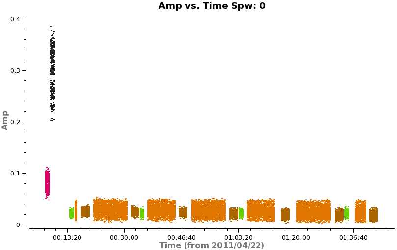
Note: when iteraxis is invoked in plotms, unzoom does not always work properly. If you have trouble with this, flip to next page and then back to current one. this usually fixes the problem.
# In CASA
plotms(vis='X3c1_wvrtsys.ms',spw='',xaxis='time',yaxis='amp',field='',avgchannel='3840',
       coloraxis='field',iteraxis='spw')
# In CASA
plotms(vis='X5d8_wvrtsys.ms',spw='',xaxis='time',yaxis='amp',field='',avgchannel='3840',
       coloraxis='field',iteraxis='spw')
# In CASA
plotms(vis='X7ef_wvrtsys.ms',spw='',xaxis='time',yaxis='amp',field='',avgchannel='3840',
       coloraxis='field',iteraxis='spw')
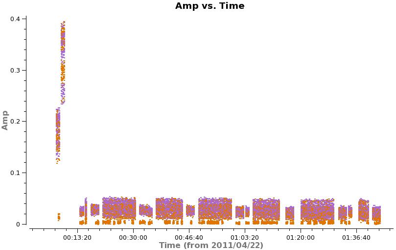
Things to Notice:
- In spw=2 there are some low points in all three data files. Use the "Mark Regions" box (left of center on bottom row of icons) to draw small box on low points. Then click the magnifying glass icon to the right of center. The output will be sent to the logger window. Note: keep the marked region small or you can overwhelm the buffer. Locate suggests correlation YY on PM03 is the culprit.
To see this more clearly you can rerun plotms with coloraxis='field' switched to coloraxis='corr'
# In CASA
plotms(vis='X3c1_wvrtsys.ms',spw='2',xaxis='time',yaxis='amp',field='',avgchannel='3840',
       coloraxis='corr')
To further check, you can exclude PM03 from the plot using antenna='!PM03'.
# In CASA
plotms(vis='X3c1_wvrtsys.ms',spw='2',xaxis='time',yaxis='amp',field='',avgchannel='3840',
       coloraxis='corr',antenna='!PM03')
Having confirmed the problem antenna, we flag it below.
# In CASA
splitdata=['X3c1_wvrtsys.ms','X5d8_wvrtsys.ms','X7ef_wvrtsys.ms']
for vis in splitdata:
  flagdata(vis=vis, flagbackup=T,
         spw=['2'],
         antenna=['PM03'],
         correlation=['YY'])
Next we need to inspect the spectral properties of the data to look for issues.
First we look at phase as a function of frequency for a well behaved antenna like DV06. coloraxis='baselines' (note this parameter is called colorize in the gui, Display Tab) will show each baseline as a different color. Significant delay errors or baseline errors will show up as phase slopes in these plots. Again you will want to page through the spectral windows.
# In CASA
plotms(vis='X3c1_wvrtsys.ms',spw='',xaxis='frequency',yaxis='phase',field='0',antenna='DV06',
       avgtime='1e8',avgscan=T,coloraxis='baseline',iteraxis='spw',xselfscale=T)
# In CASA
plotms(vis='X5d8_wvrtsys.ms',spw='',xaxis='frequency',yaxis='phase',field='0',antenna='DV06',
       avgtime='1e8',avgscan=T,coloraxis='baseline',iteraxis='spw',xselfscale=T)
# In CASA
plotms(vis='X7ef_wvrtsys.ms',spw='',xaxis='frequency',yaxis='phase',field='0',antenna='DV06',
       avgtime='1e8',avgscan=T,coloraxis='baseline',iteraxis='spw',xselfscale=T)
Overall these plots look good with no large delays or baseline errors apparent.
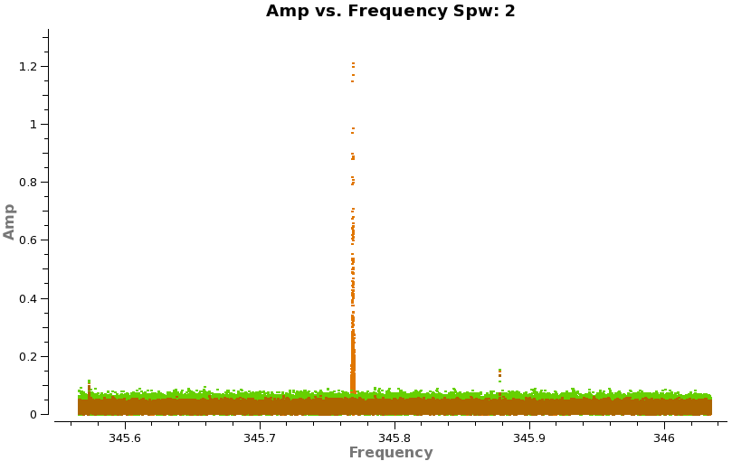
With such high spectral resolution data, one often sees occasional "birdies" in the data. These are typically very narrow weak spectral features that are internally generated in the system. Over time as we track down issues the number of birdies should decrease, but you should always check. This is easiest to do by looking at amplitude vs. frequency for sources observed over a long time range (for sensitivity). It is helpful to look at more than one source to verify the nature of the emission. Below we look at both calibrators (brown and green) and TW Hya (orange). If you have enough sensitivity birdies should be seen on all sources, however, be careful not to mistake real line emission for a birdie even on a calibrator - they can be present as we've seen for Titan.
# In CASA
plotms(vis='X3c1_wvrtsys.ms',spw='',xaxis='channel',yaxis='amp',field='2,3,4',
       avgtime='1e8',avgscan=T,coloraxis='field',iteraxis='spw',xselfscale=T,yselfscale=T)
Do a quick check that other two datasets are the same (they are usually similar if the source of internal resonance hasn't changed in the meantime).
# In CASA
plotms(vis='X5d8_wvrtsys.ms',spw='',xaxis='channel',yaxis='amp',field='2,3,4',
       avgtime='1e8',avgscan=T,coloraxis='field',iteraxis='spw',xselfscale=T,yselfscale=T)
# In CASA
plotms(vis='X7ef_wvrtsys.ms',spw='',xaxis='channel',yaxis='amp',field='2,3,4',
       avgtime='1e8',avgscan=T,coloraxis='field',iteraxis='spw',xselfscale=T,yselfscale=T)
Now you can zoom in on each region to get channels for flagging, or to save time just go ahead and run the flagging command below where this has been done for you.
# In CASA
splitdata=['X3c1_wvrtsys.ms','X5d8_wvrtsys.ms','X7ef_wvrtsys.ms']
for vis in splitdata:
  flagdata(vis=vis, flagbackup=T,
         spw=['0:1067~1068;1279~1280;2367~2368;3775~3776',
              '1:1279~1280;2367~2368;3775~3776',
              '2:1279~1280;3775~3776',
              '3:831~832;1535~1536;2367~2368;3775~3776;3839~3839'])
Replot in plotms to check that flagging has been done as anticipated.
Flag Calibrator Spectral Features
In this section, we will flag spectral features in the calibrators so they do not skew the calibration solutions. First make plots of 3C279 and Titan in channel space to get channels for flagging.
# In CASA
basename=["X3c1_wvrtsys","X5d8_wvrtsys","X7ef_wvrtsys"]
for asdm in basename:
  plotms(vis=asdm+'.ms',spw='',xaxis='channel',yaxis='amp',field='0,1',
         avgtime='1e8',coloraxis='field',iteraxis='spw')
  print('When you are done with the graphics window,')
  print('quit that window, and')
  user_check=raw_input('press enter to continue script\n')
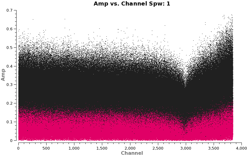
The figure to the right shows a broad absorption line in spw 1 at channel 3000. This is the ozone absorption line at 357.62982 GHz. However, there is another narrow absorption feature in the spectra (spw 2) that is most easily seen on 3C279 (because it is the strongest calibrator). Let's look at it first in frequency space.
# In CASA
for asdm in basename:
  plotms(vis=asdm+'.ms',spw='2:1600~2300',xaxis='frequency',yaxis='amp',
         field='0',avgtime='1e8',coloraxis='field')
  print('When you are done with the graphics window,')
  print('quit that window, and')
  user_check=raw_input('press enter to continue script\n')
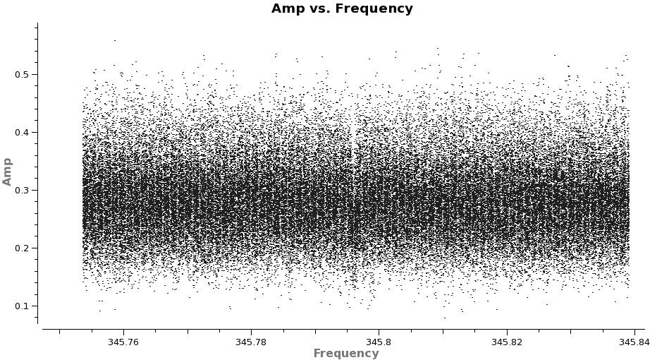
The absorption feature lies exactly at the rest frequency for CO 3-2 (345.79599 GHz). Because it is so narrow (< 1 MHz), it must originate from a very low pressure region (i.e. high altitude) in the Earth's atmosphere, otherwise it would be more pressure broadened. Indeed, the first detection of CO in the mesosphere was made over 35 years ago (see, e.g. Waters et al. 1976 or Goldsmith et al. 1979). Be aware that the line is stronger as you go up the CO ladder (strength ~ J^3 for low J) because the temperature at that altitude (~50km) is about 250 K. In April 2011, the apparent depth of the feature was about 10% in the 2-1 line and 35% in the 3-2 line. However, the depth of the absorption feature is exaggerated due to the way ALMA normalizes the cross-correlation spectra by the autocorrelation spectra prior to storage. While this technique generally leads to a flat bandpass shape, it will accentuate telluric features because they are emission lines in the single dish spectrum (e.g. JCMT observations of mesospheric CO 3-2 can be found in Preston et al. 1993). Finally, note that large seasonal variations in the line strength have been reported from observations at Onsala.
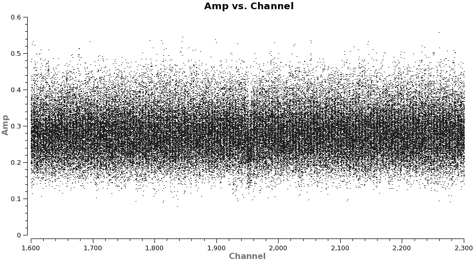
Now, let's re-plot the line with channel number as the x-axis in order to get the channel range for flagging.
# In CASA
for asdm in basename:
  plotms(vis=asdm+'.ms',spw='2:1600~2300',xaxis='channel',yaxis='amp',
         field='0',avgtime='1e8',coloraxis='field')
  print('When you are done with the graphics window,')
  print('quit that window, and')
  user_check=raw_input('press enter to continue script\n')
Now lets look at Titan in more detail.
# In CASA
for asdm in basename:
  plotms(vis=asdm+'.ms',spw='',xaxis='channel',yaxis='amp',field='1',
         avgtime='1e8',coloraxis='field',iteraxis='spw')
  print('When you are done with the graphics window,')
  print('quit that window, and')
  user_check=raw_input('press enter to continue script\n')
Explicitly back up the flag tables so that flagged regions can be restored later.
# In CASA
for asdm in basename:
  flagmanager(vis=asdm+'.ms',mode='save',versionname=asdm+'.before_calspectralflags')
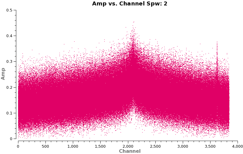
Flag absorption features for all sources.
# In CASA
for asdm in basename:
  print "Flagging absorption features in all sources for "+asdm
  flagdata(vis=asdm+'.ms', spw=['1:2000~3840','2:1945~1960'])
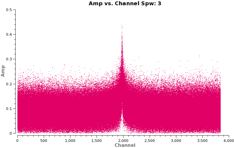
Now we need to flag emission. The very broad CO(3-2) in spw=2 of Titan will prevent us from using it as a calibrator for this spectral window since there are no line-free channels (we will transfer, phase, amplitude, and absolute flux from another Titan spw below). We do want to flag the narrower Titan line in spw=3.
# In CASA
for asdm in basename:
  flagmanager(vis=asdm+'.ms',mode='save',versionname=asdm+'.before_emissionflags')
# In CASA
for asdm in basename:
  print "Flagging emission for "+asdm
  flagdata(vis=asdm+'.ms',
           field=['1'],
           spw=['3:1000~3000'])
If you like, check that the right things have been flagged.
# In CASA
for asdm in basename:
  plotms(vis=asdm+'.ms',spw='',xaxis='channel',yaxis='amp',field='0,1',
         avgtime='1e8',coloraxis='field',iteraxis='spw')
  print('When you are done with the graphics window,')
  print('quit that window, and')
  user_check=raw_input('press enter to continue script\n')
Set Up the Flux Calibrator Model
Fill the model data column for Titan with a model for the flux density as a function of baseline. The model is a uniformly illuminated disk with the size obtained from the JPL Horizons ephemeris.
# In CASA
basename=["X3c1_wvrtsys","X5d8_wvrtsys","X7ef_wvrtsys"]
for asdm in basename:
  setjy(vis=asdm+'.ms',field='1',
        standard='Butler-JPL-Horizons 2010',scalebychan=F)
Bandpass Calibration


First we need to check how the amplitude and phase of 3C279 behave as a function of time.
# In CASA
for asdm in basename:
  plotms(vis=asdm+'.ms',spw='',xaxis='time',yaxis='amp',
         field='0',avgchannel='3840',iteraxis='spw')
  print('When you are done with the graphics window,')
  print('quit that window, and')
  user_check=raw_input('press enter to continue script\n')
Page through the spws. This shows significant variations in the amplitude across the three scans.
# In CASA
for asdm in basename:
  plotms(vis=asdm+'.ms',spw='0',xaxis='time',yaxis='phase',
         antenna='DV06;!DV04',coloraxis='corr',
         field='0',avgchannel='3840',iteraxis='baseline')
  print('When you are done with the graphics window,')
  print('quit that window, and')
  user_check=raw_input('press enter to continue script\n')
Page through the baselines to DV06. This examination reveals two findings: (1) significant variation in the phase across the three scans, as well as (2) smaller but significant variations within a scan. The first finding suggests that we do not want to combine the scans for bandpass calibration, but instead derive an independent bandpass for each scan. Actually what is more important than a DC offset is if the shape of the amplitude or phase changes from scan to scan. There isn't enough S/N to tell for sure so we will keep them separate. The second finding suggests that we need to correct the phase vs. time behavior of the bandpass calibrator (3C279; field=0) within each scan, before doing the bandpass. We want to chose a relatively narrow range of channels near the center of the spws so that the bandpass phase slopes (to be corrected with the bandpass calibration itself) do not decorrelate the signal. You need to avoid spectral regions that were completely flagged above.
# In CASA
for asdm in basename:
  gaincal(vis=asdm+'.ms',caltable=asdm+'.bpphase.gcal',
          field='0',spw='0~3:900~1100',refant='DV06',
          calmode='p',solint='int',minsnr=2.0,minblperant=4)
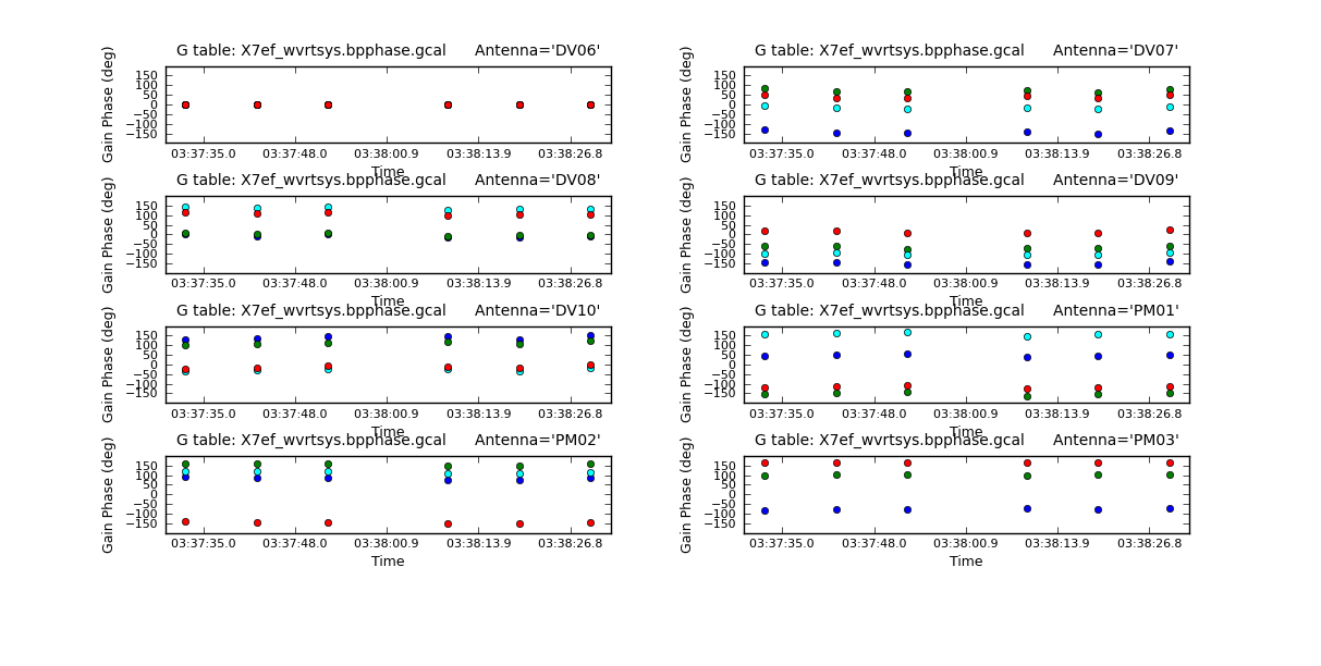
Inspect the phase-only calibration solutions for the bandpass calibrator. Look for any noisy solutions. We do XX and YY separately to reduce confusion in the plot. It will help if you make your plotcal window wide.
# In CASA
for asdm in basename:
  plotcal(caltable=asdm+'.bpphase.gcal',xaxis='time',yaxis='phase',spw='',antenna='1~8',
          iteration='antenna',subplot=421,plotrange=[0,0,-180,180],
          figfile=asdm+'.bpphase.X.png',poln='X')
  print('When you are done with the graphics window,')
  print('quit that window, and')
  user_check=raw_input('press enter to continue script\n')
In the plotcal gui you can use the magnifying glass symbol to zoom in on one of the scans to see the phase variations. The colors are the 4 different spws.
# In CASA
for asdm in basename:
  plotcal(caltable=asdm+'.bpphase.gcal',xaxis='time',yaxis='phase',spw='',antenna='1~8',
          iteration='antenna',subplot=421,plotrange=[0,0,-180,180],
          figfile=asdm+'.bpphase.Y.png',poln='Y')
  print('When you are done with the graphics window,')
  print('quit that window, and')
  user_check=raw_input('press enter to continue script\n')
Next we apply this phase-only correction on the fly while calculating the bandpass solutions.
# In CASA
for asdm in basename:
  bandpass(vis=asdm+'.ms',caltable=asdm+'.bandpass.bcal',
           field='0',spw='',combine='',refant='DV06',
           solint='inf',solnorm=T,minblperant=4,fillgaps=17,
           gaintable=[asdm+'.bpphase.gcal'])
You will see some error messages, these are just related to the flagged channels. We set fillgaps=17 to interpolate across the smaller regions of flagged channels (mesospheric features and birdies).
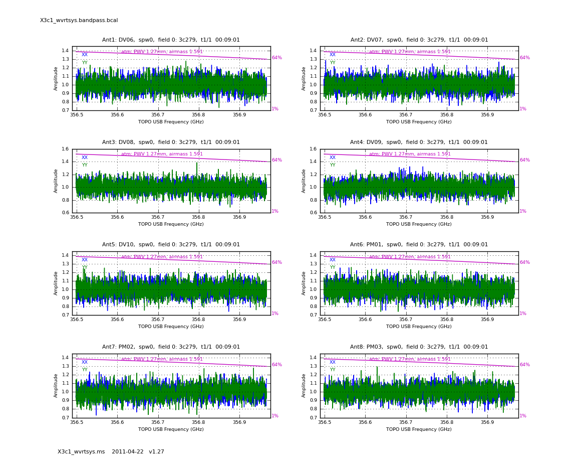
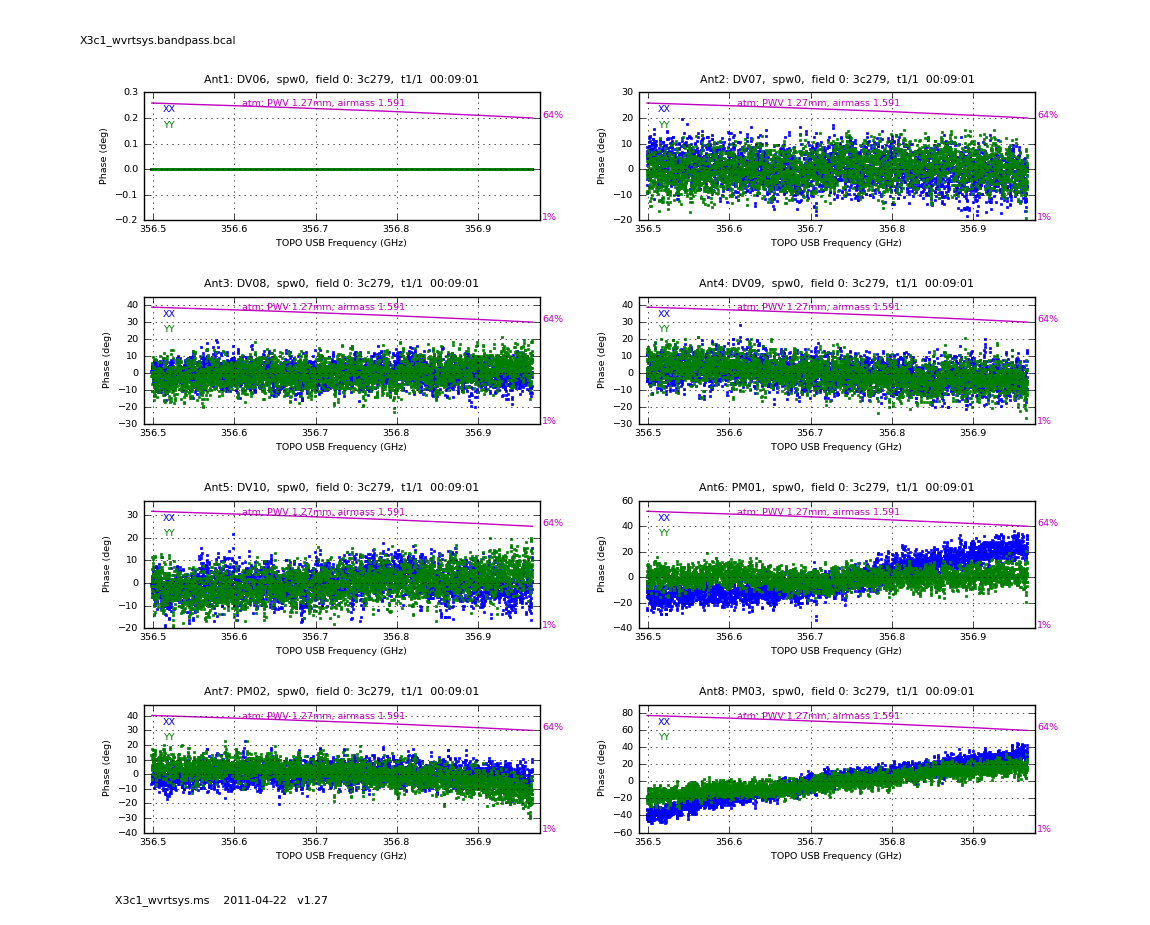
A few words about solint and combine:
In bandpass, the use of solint='inf' (as in "infinite") will derive a bandpass solution for each 3C279 scan, unless combine='scan' (which is the default). Here we set combine=' ' explicitly so that it does not combine the scans into one bandpass. Likewise, field boundaries are only crossed if combine='field', and spw boundaries are only crossed if combine='spw'. In some cases it can be helpful to combine fields if you suffer from lack of S/N, but it is never a good idea to combine spws.
Now inspect the phase and amplitude solutions. You are looking for excursions from smooth fits, or particularly noisy solutions compared to the others. These plots take a while because there are so many channels per spw (3840!).
# In CASA
for asdm in basename:
  plotcal(caltable=asdm+'.bandpass.bcal',xaxis='freq',yaxis='amp',antenna='1~8',
          iteration='antenna',subplot=421,spw='0',figfile=asdm+'.bandpass.ampspw0.png')
  print('When you are done with the graphics window,')
  print('quit that window, and')
  user_check=raw_input('press enter to continue script\n')
# In CASA
for asdm in basename:
  plotcal(caltable=asdm+'.bandpass.bcal',xaxis='freq',yaxis='phase',antenna='1~8',
          iteration='antenna',subplot=421,spw='0',figfile=asdm+'.bandpass.phasespw0.png')
  print('When you are done with the graphics window,')
  print('quit that window, and')
  user_check=raw_input('press enter to continue script\n')
The values of phase on DV06 are very small because it was used as the reference antenna.
These plots should be repeated for each spw. Be sure to rename the plot's file each time before running.
Gain Calibration
Now that we have a bandpass solution to apply we can solve for the antenna-based phase and amplitude gain calibration. Since the phase changes on a much shorter timescale than the amplitude, we will solve for them separately. In particular, if the phase changes significantly over a scan time, the amplitude would be decorrelated, if the un-corrected phase were averaged over this timescale. Note that we re-solve for the gain solutions of the bandpass calibrator, so we can derive new solutions that are corrected for the bandpass shape. Since the bandpass calibrator will not be used again, this is not strictly necessary, but is useful to check its calibrated flux density for example.
# In CASA
basename=["X3c1_wvrtsys","X5d8_wvrtsys","X7ef_wvrtsys"]
for asdm in basename:
  gaincal(vis=asdm+'.ms',caltable=asdm+'.intphase.gcal',
          field='0,1,3,4',spw='0~3:40~3800',refant='DV06',
          calmode='p',solint='int',minsnr=2.0,minblperant=4,
          gaintable=[asdm+'.bandpass.bcal'])
Here solint='int' coupled with calmode='p' will derive a single phase solution for each 10 second integration. Note that the bandpass table is applied on-the-fly before solving for the phase solutions, however the bandpass is NOT applied to the data permanently until applycal is run later on.
Although solint='int' (i.e. the integration time of 10 seconds) is the best choice to apply before for solving for the amplitude solutions, it is not a good idea to use this to apply to the target. This is because the phase-scatter within a scan can dominate the interpolation between calibrator scans. Instead, we also solve for the phase on the scan time, solint='inf' (but combine=' ', since we want one solution per scan) for application to the target later on. Unlike the bandpass task, for gaincal, the default of the combine parameter is combine=' '.
# In CASA
for asdm in basename:
  gaincal(vis=asdm+'.ms',caltable=asdm+'.scanphase.gcal',
          field='0,1,3,4',spw='0~3:40~3800',refant='DV06',
          calmode='p',solint='inf',minsnr=2.0,minblperant=4,
          gaintable=[asdm+'.bandpass.bcal'])
Alternatively, instead of making a separate phase solution for application to the target, one can also run smoothcal to smooth the solutions derived on the integration time.
Next we apply the bandpass and solint='int' phase-only calibration solutions on-the-fly to derive amplitude solutions. Here the use of solint='inf', but combine=' ' will result in one solution per scan interval.
# In CASA
for asdm in basename:
  gaincal(vis=asdm+'.ms',caltable=asdm+'.amp.gcal',
          field='0,1,3,4',spw='0~3:40~3800',refant='DV06',
          calmode='ap',solint='inf',minsnr=2.0,minblperant=4,
          gaintable=[asdm+'.bandpass.bcal',asdm+'.intphase.gcal'])
Now carefully inspect all these solutions looking for discrepant solutions. If you see any, you will need to flag them and rerun the calibration tasks above.
We make plots in X and Y separately for clarity. The colors are showing the spectral windows.
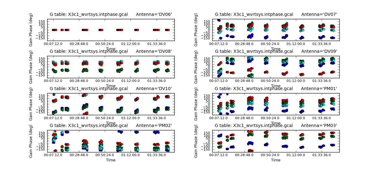
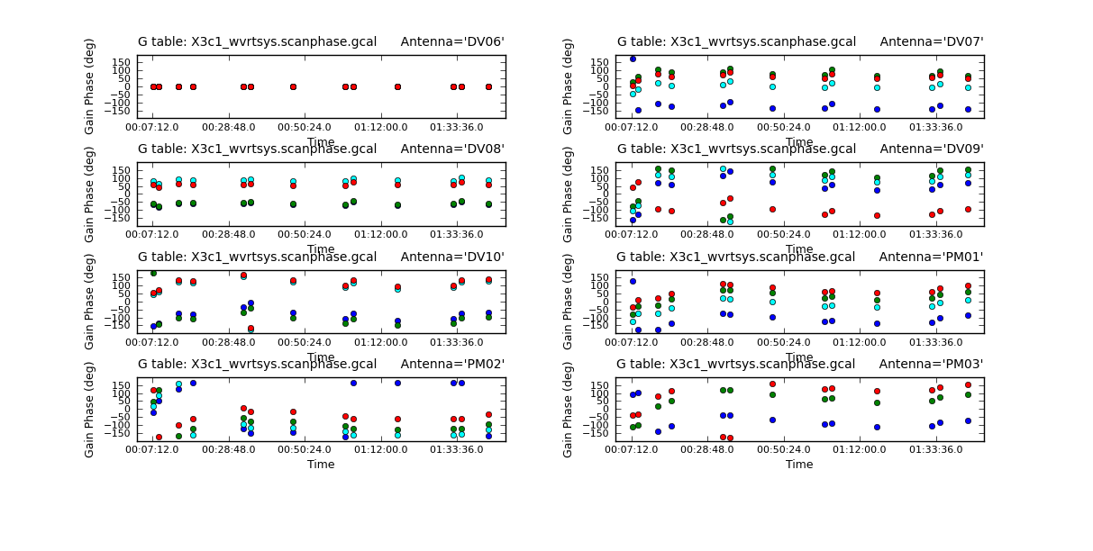
# In CASA
for asdm in basename:
  plotcal(caltable=asdm+'.intphase.gcal',xaxis='time',yaxis='phase',antenna='1~8',
          spw='',field='0,1,3,4',iteration='antenna',subplot=421,
          plotrange=[0,0,-180,180],poln='X',figfile=asdm+'.intphase_X.png')
  print('When you are done with the graphics window,')
  print('quit that window, and')
  user_check=raw_input('press enter to continue script\n')
# In CASA
for asdm in basename:
  plotcal(caltable=asdm+'.intphase.gcal',xaxis='time',yaxis='phase',antenna='1~8',
          spw='',field='0,1,3,4',iteration='antenna',subplot=421,
          plotrange=[0,0,-180,180],poln='Y',figfile=asdm+'.intphase_Y.png')
  print('When you are done with the graphics window,')
  print('quit that window, and')
  user_check=raw_input('press enter to continue script\n')
# In CASA
for asdm in basename:
  plotcal(caltable=asdm+'.scanphase.gcal',xaxis='time',yaxis='phase',antenna='1~8',
          spw='',field='0,1,3,4',iteration='antenna',subplot=421,
          plotrange=[0,0,-180,180],poln='X',figfile=asdm+'.scanphase_X.png')
  print('When you are done with the graphics window,')
  print('quit that window, and')
  user_check=raw_input('press enter to continue script\n')
# In CASA
for asdm in basename:
  plotcal(caltable=asdm+'.scanphase.gcal',xaxis='time',yaxis='phase',antenna='1~8',
          spw='',field='0,1,3,4',iteration='antenna',subplot=421,
          plotrange=[0,0,-180,180],poln='Y',figfile=asdm+'.scanphase_Y.png')
  print('When you are done with the graphics window,')
  print('quit that window, and')
  user_check=raw_input('press enter to continue script\n')
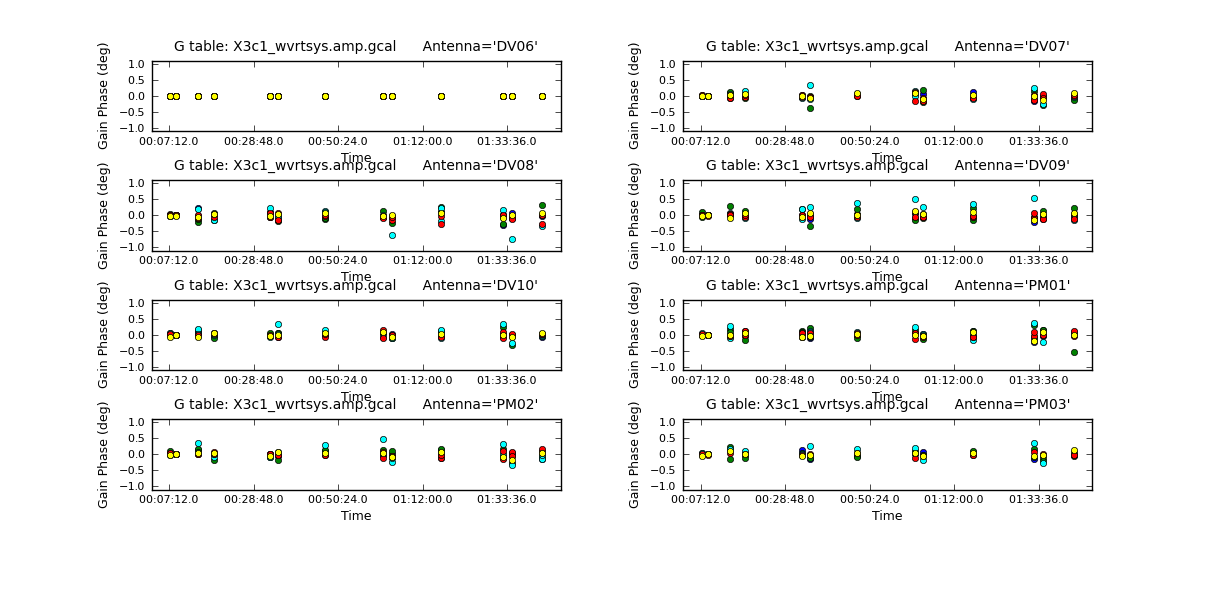
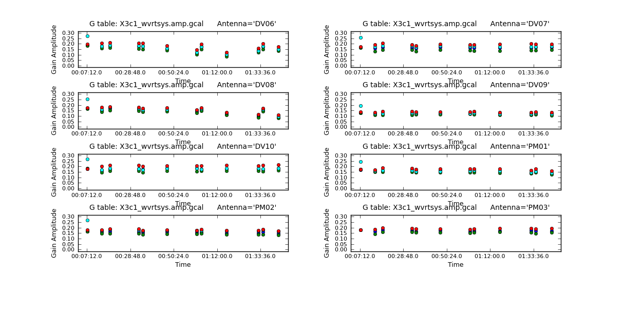
Since we have taken out the phase as best we can by applying the solint='int' phase-only solution, this plot will give a good idea of the residual phase error. If you see scatter of more than a few degrees here, you should consider going back and looking for more data to flag, particularly bad timeranges etc.
# In CASA
for asdm in basename:
  plotcal(caltable=asdm+'.amp.gcal',xaxis='time',yaxis='phase',antenna='1~8',
          spw='',field='0,1,3,4',plotrange=[0,0,-1,1],
          iteration='antenna',subplot=421,figfile=asdm+'.amp_phase.png')
  print('When you are done with the graphics window,')
  print('quit that window, and')
  user_check=raw_input('press enter to continue script\n')
These are very small, as they should be. Now look at the amplitude solutions.
# In CASA
for asdm in basename:
  plotcal(caltable=asdm+'.amp.gcal',xaxis='time',yaxis='amp',antenna='1~8',
          iteration='antenna',subplot=421,spw='',poln='X',
          plotrange=[0,0,0.0,0.3],figfile=asdm+'.amp_X.png')
  print('When you are done with the graphics window,')
  print('quit that window, and')
  user_check=raw_input('press enter to continue script\n')
# In CASA
for asdm in basename:
  plotcal(caltable=asdm+'.amp.gcal',xaxis='time',yaxis='amp',antenna='1~8',
          iteration='antenna',subplot=421,spw='',poln='Y',
          plotrange=[0,0,0.0,0.3],figfile=asdm+'.amp_Y.png')
  print('When you are done with the graphics window,')
  print('quit that window, and')
  user_check=raw_input('press enter to continue script\n')
Flux Calibration
Next we use the flux calibrator (whose flux density was set in setjy above) to derive the flux of the other calibrators. Note that the flux table REPLACES the amp.gcal in terms of future application of the calibration to the data, i.e. the flux table contains both the amp.gcal and flux scaling. Unlike the gain calibration steps, this is not an incremental table.
# In CASA
for asdm in basename:
  fluxscale(vis=asdm+'.ms',caltable=asdm+'.amp.gcal',
            fluxtable=asdm+'.flux.cal',reference='1',refspwmap=[0,1,3,3])
Its a good idea to note down the derived fluxscale values for your records. This can be found in the Log Messages window.
 Found reference field(s): Titan
 Found transfer field(s):  3c279 J1147-382=QSO J1037-295=QSO
 Spw=2 will be referenced to spw=3
 Flux density for 3c279 in SpW=0 is: 10.7324 +/- 0.180055 (SNR = 59.6062, nAnt= 8)
 Flux density for 3c279 in SpW=1 is: 10.953 +/- 0.163625 (SNR = 66.9394, nAnt= 8)
 Flux density for 3c279 in SpW=2 (ref SpW=3) is: 10.7283 +/- 0.191615 (SNR = 55.9888, nAnt= 7)
 Flux density for 3c279 in SpW=3 is: 10.1286 +/- 0.143758 (SNR = 70.4556, nAnt= 8)
 Flux density for J1147-382=QSO in SpW=0 is: 0.913886 +/- 0.0106354 (SNR = 85.9287, nAnt= 8)
 Flux density for J1147-382=QSO in SpW=1 is: 0.734573 +/- 0.00852182 (SNR = 86.1991, nAnt= 8)
 Flux density for J1147-382=QSO in SpW=2 (ref SpW=3) is: 0.917729 +/- 0.0101124 (SNR = 90.7532, nAnt= 7)
 Flux density for J1147-382=QSO in SpW=3 is: 1.12946 +/- 0.0130193 (SNR = 86.7525, nAnt= 8)
 Flux density for J1037-295=QSO in SpW=0 is: 0.890222 +/- 0.00878729 (SNR = 101.308, nAnt= 8)
 Flux density for J1037-295=QSO in SpW=1 is: 0.708348 +/- 0.00675153 (SNR = 104.917, nAnt= 8)
 Flux density for J1037-295=QSO in SpW=2 (ref SpW=3) is: 0.896367 +/- 0.00856783 (SNR = 104.62, nAnt= 7)
 Flux density for J1037-295=QSO in SpW=3 is: 1.11563 +/- 0.0102939 (SNR = 108.378, nAnt= 8)
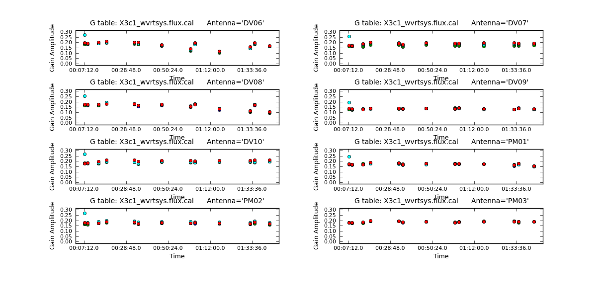
Now look at the flux solutions.
# In CASA
for asdm in basename:
  plotcal(caltable=asdm+'.flux.cal',xaxis='time',yaxis='amp',antenna='1~8',
          iteration='antenna',subplot=421,spw='',poln='X',
          plotrange=[0,0,0.0,0.3],figfile=asdm+'.flux_X.png')
  print('When you are done with the graphics window,')
  print('quit that window, and')
  user_check=raw_input('press enter to continue script\n')
# In CASA
for asdm in basename:
  plotcal(caltable=asdm+'.flux.cal',xaxis='time',yaxis='amp',antenna='1~8',
          iteration='antenna',subplot=421,spw='',poln='Y',
          plotrange=[0,0,0.0,0.3],figfile=asdm+'.flux_Y.png')
  print('When you are done with the graphics window,')
  print('quit that window, and')
  user_check=raw_input('press enter to continue script\n')
Apply Calibration and Inspect
Now we can use the flagmanager if we want to restore any of the spectral flagging we did prior to bandpass calibration. In this case, we choose to restore the flags of the emission lines on Titan, because we are interested in seeing how strong they are compared to the continuum. However, we leave the strong ozone line and mesospheric CO line flagged on all sources, because we want to get the most accurate continuum flux density for the science target.
# In CASA
basename=["X3c1_wvrtsys","X5d8_wvrtsys","X7ef_wvrtsys"]
for asdm in basename:
  flagmanager(vis=asdm+'.ms',mode='restore',versionname=asdm+'.before_emissionflags')
Next we apply the calibration solutions to each source individually, using the gainfield parameter to specify which calibrators solutions should be applied from each of the gaintable calibration tables.
First, we do 3C279 (the bandpass calibrator), applying all 3 of its solutions to itself (that's why gainfield contains three zeros):
# In CASA
for asdm in basename:
  applycal(vis=asdm+'.ms',field='0',
           gaintable=[asdm+'.bandpass.bcal',asdm+'.intphase.gcal',asdm+'.flux.cal'],
           interp=['nearest','nearest','nearest'],
           gainfield=['0','0','0'],flagbackup=T)
Next, we do Titan (the absolute flux calibrator) using the bandpass solution from 3C279:
# In CASA
for asdm in basename:
  applycal(vis=asdm+'.ms',field='1',
           gaintable=[asdm+'.bandpass.bcal',asdm+'.intphase.gcal',asdm+'.flux.cal'],
           interp=['nearest','nearest','nearest'],
           gainfield=['0','1','1'], flagbackup=T, calwt=F)
For the secondary phase calibrator, we apply the phase and flux solutions from the primary phase calibrator. This will allow us to independently assess how well the phase transfer to the science target (TW Hya) has worked:
# In CASA
for asdm in basename:
  applycal(vis=asdm+'.ms',field='3',
           gaintable=[asdm+'.bandpass.bcal',asdm+'.scanphase.gcal',asdm+'.flux.cal'],
           interp=['nearest','linear','linear'],
           gainfield=['0','4','4'], flagbackup=T, calwt=F)
Next is the Primary phase calibrator:
# In CASA
for asdm in basename:
  applycal(vis=asdm+'.ms',field='4',
           gaintable=[asdm+'.bandpass.bcal',asdm+'.intphase.gcal',asdm+'.flux.cal'],
           interp=['nearest','nearest','nearest'],
           gainfield=['0','4','4'], flagbackup=T, calwt=F)
Finally, for the Science Target TW Hya, we apply the phase solutions from both the primary and secondary phase calibrators:
# In CASA
for asdm in basename:
  applycal(vis=asdm+'.ms',field='2',
           interp=['nearest','linear','linear'],
           gaintable=[asdm+'.bandpass.bcal',asdm+'.scanphase.gcal',asdm+'.flux.cal'],
           gainfield=['0','3,4','3,4'], flagbackup=T, calwt=F)
Now we can check the results of applying the calibration solutions.
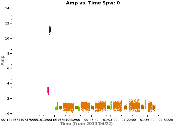
# In CASA
for asdm in basename:
  plotms(vis=asdm+'.ms',spw='',xaxis='time',yaxis='amp',field='',avgchannel='3840',
         coloraxis='field',iteraxis='spw',ydatacolumn='corrected')
  print('When you are done with the graphics window,')
  print('quit that window, and')
  user_check=raw_input('press enter to continue script\n')
In amplitude, it looks good but there are some noisy points toward the end of the first scheduling block, but it mostly only affects the secondary phase calibrator (green). In phase, we expect all the points to cluster about zero. The large scatter in phase on the secondary phase calibrator is readily apparent:
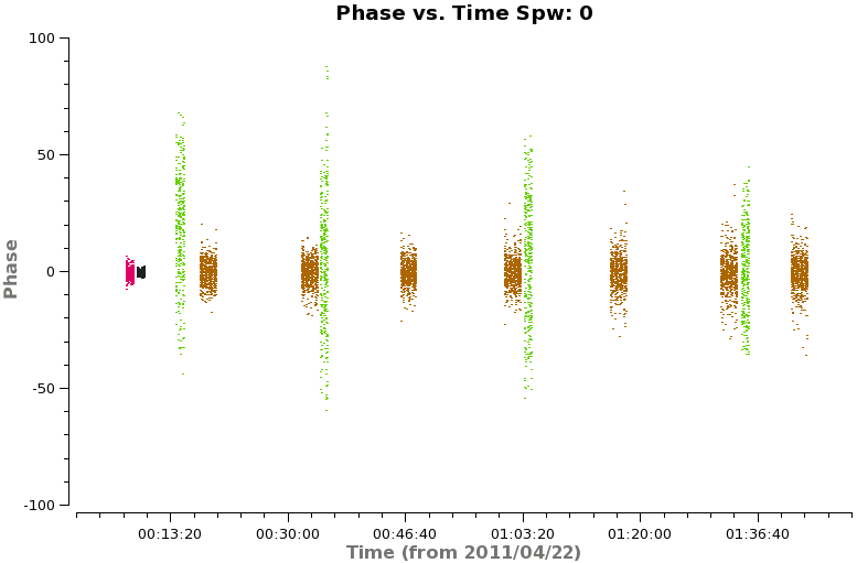
# In CASA
for asdm in basename:
  plotms(vis=asdm+'.ms',spw='',xaxis='time',yaxis='phase',field='0,1,3,4',avgchannel='3840',
         coloraxis='field',iteraxis='spw',ydatacolumn='corrected')
  print('When you are done with the graphics window,')
  print('quit that window, and')
  user_check=raw_input('press enter to continue script\n')
Let's check whether the situation improves when we apply this calibrator's solutions to itself rather than transferring the solutions from the primary phase calibrator (which is 17 degrees away, and observed at a different time).
# In CASA
for asdm in basename:
  applycal(vis=asdm+'.ms',field='3',
           gaintable=[asdm+'.bandpass.bcal',asdm+'.intphase.gcal',asdm+'.flux.cal'],
           interp=['nearest','nearest','nearest'],
           gainfield=['0','3','3'], flagbackup=T, calwt=F)
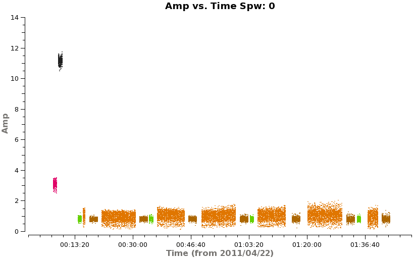
# In CASA
for asdm in basename:
  plotms(vis=asdm+'.ms',spw='',xaxis='time',yaxis='amp',field='',avgchannel='3840',
         coloraxis='field',iteraxis='spw',ydatacolumn='corrected')
  print('When you are done with the graphics window,')
  print('quit that window, and')
  user_check=raw_input('press enter to continue script\n')
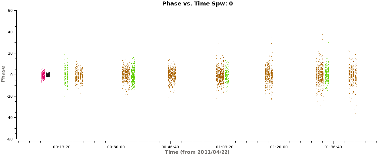
# In CASA
for asdm in basename:
  plotms(vis=asdm+'.ms',spw='',xaxis='time',yaxis='phase',field='0,1,3,4',avgchannel='3840',
         coloraxis='field',iteraxis='spw',ydatacolumn='corrected')
  print('When you are done with the graphics window,')
  print('quit that window, and')
  user_check=raw_input('press enter to continue script\n')
Indeed, the secondary calibrator looks better now in amplitude and phase. This is an indication that the calibration transfer is not working well in this timerange. Because the effect is not catastrophic and we know we can self-calibrate on TW Hya later, we will let this go for now. Or if you want you can delve deeper into the data and try to solve the mystery... In any case, so that we can later check the effect of correcting the secondary phase calibrator with the primary phase calibrator, we will re-issue the original applycal so that it is this calibration that our subsequent split will use.
# In CASA
for asdm in basename:
  applycal(vis=asdm+'.ms',field='3',
           gaintable=[asdm+'.bandpass.bcal', asdm+'.scanphase.gcal', asdm+'.flux.cal'],
           interp=['nearest','linear','linear'],
           gainfield=['0','4','4'], flagbackup=T, calwt=F)
Let's examine the spectral calibration now. First, 3C279 and Titan:
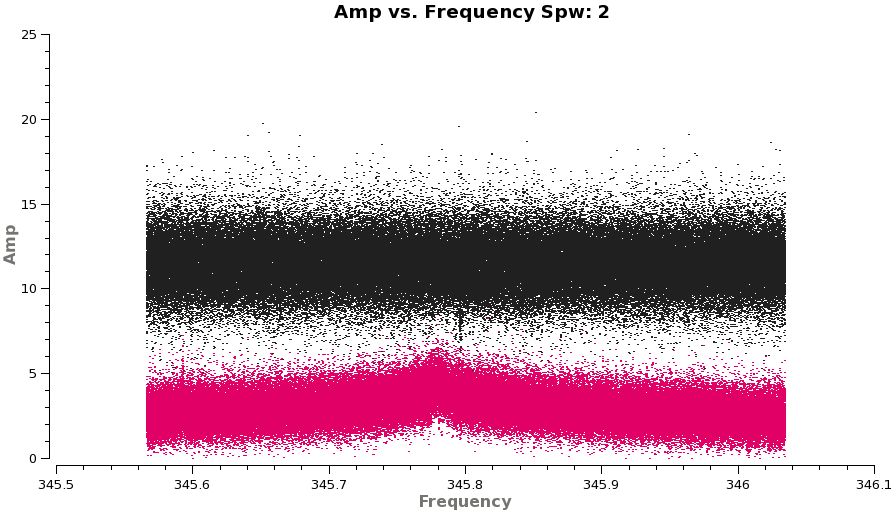
# In CASA
for asdm in basename:
  plotms(vis=asdm+'.ms',spw='',xaxis='frequency',yaxis='amp',field='0,1',
         avgtime='1e8',avgscan=T,coloraxis='field',ydatacolumn='corrected',
         iteraxis='spw',xselfscale=T)
  print('When you are done with the graphics window,')
  print('quit that window, and')
  user_check=raw_input('press enter to continue script\n')
Flip through the spws. These look good. Next the two phase calibrators:
# In CASA
for asdm in basename:
  plotms(vis=asdm+'.ms',spw='',xaxis='frequency',yaxis='amp',field='3,4',
         avgtime='1e8',avgscan=T,coloraxis='field',ydatacolumn='corrected',
         iteraxis='spw',xselfscale=T)
  print('When you are done with the graphics window,')
  print('quit that window, and')
  user_check=raw_input('press enter to continue script\n')
Flip through the spws. This also looks good, the secondary phase calibrator is a bit noisier but this is normal. The upswing at the lower frequency end of spw=3 will probably need to be flagged on the science target as well. It corresponds to the edge of an atmospheric feature.
Now for the exciting part, what does the science target look like...
# In CASA
for asdm in basename:
  plotms(vis=asdm+'.ms',spw='',xaxis='frequency',yaxis='amp',field='2',
         avgtime='1e8',avgscan=T,coloraxis='field',ydatacolumn='corrected',
         iteraxis='spw',xselfscale=T)
  print('When you are done with the graphics window,')
  print('quit that window, and')
  user_check=raw_input('press enter to continue script\n')
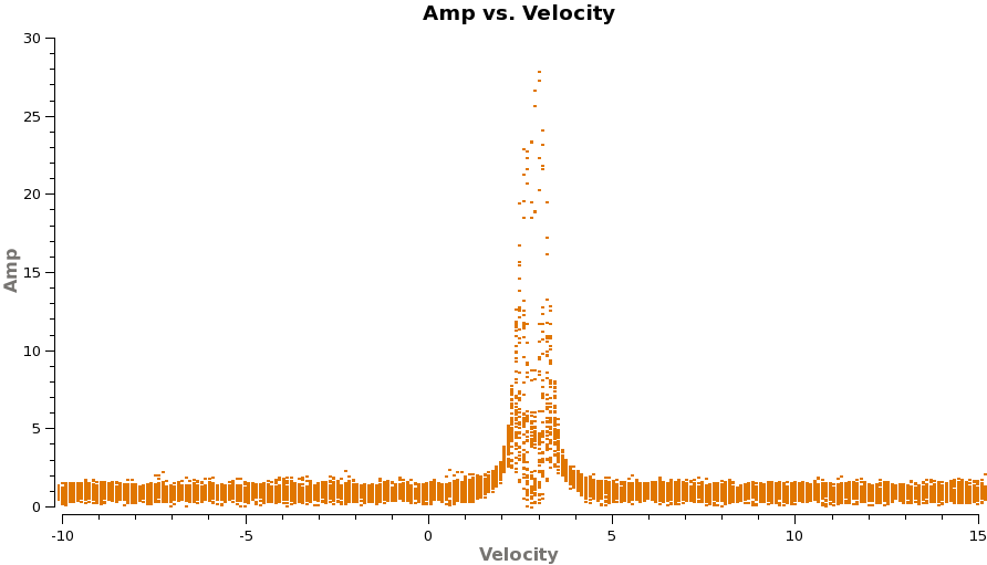
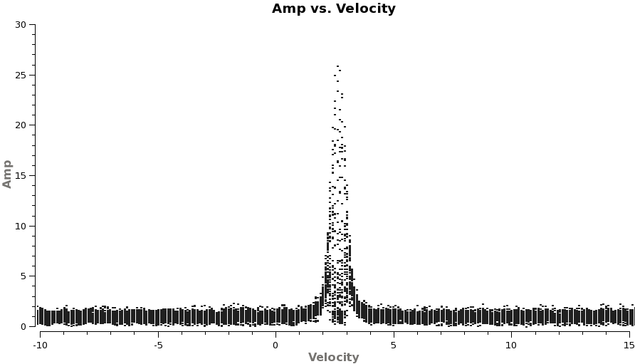
We see HCO+(4-3) in spw=0 and CO(3-2) in spw=2 as expected. Because the shape of the line profiles varies with baseline, you can already tell that the line emission is resolved.
Now check that the velocity of TWHydra is correct in the LSRK frame, it should be around 2.88 km/s.
- CO 3-2 rest freq 345.79599 GHz
- HCO+ 4-3 rest freq 356.7342 GHz
# In CASA
for asdm in basename:
  plotms(vis=asdm+'.ms',spw='2',xaxis='velocity',yaxis='amp',field='2',
         avgtime='1e8',avgscan=T,transform=T,freqframe='LSRK',restfreq='345.79599GHz',
         plotrange=[-10,15,0,0],coloraxis='spw')
  print('When you are done with the graphics window,')
  print('quit that window, and')
  user_check=raw_input('press enter to continue script\n')
# In CASA
for asdm in basename:
  plotms(vis=asdm+'.ms',spw='0',xaxis='velocity',yaxis='amp',field='2',
         avgtime='1e8',avgscan=T,transform=T,freqframe='LSRK',restfreq='356.7342GHz',
         plotrange=[-10,15,0,0],coloraxis='spw')
  print('When you are done with the graphics window,')
  print('quit that window, and')
  user_check=raw_input('press enter to continue script\n')
Both lines show up at the expected velocity.
Concatenate the Data
Here we will concatenate the three calibrated datasets prior to imaging.
# In CASA
splitdata=['X3c1_wvrtsys.ms','X5d8_wvrtsys.ms','X7ef_wvrtsys.ms']
os.system('rm -rf Band7multi_april22.ms')
concat(vis=splitdata,concatvis='Band7multi_april22.ms')
If you like you can run listobs on new combined dataset:
# In CASA
listobs(vis='Band7multi_april22.ms',verbose=F)
You can also examine the spectral uv plots for the combined dataset to see the improvement in S/N:
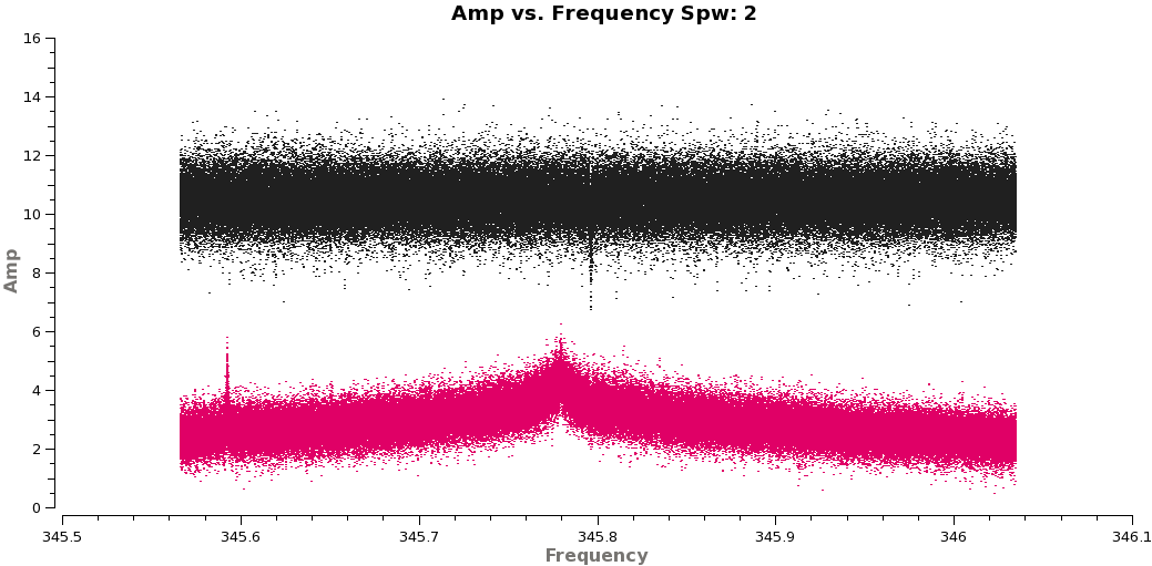
# In CASA
for asdm in basename:
  plotms(vis='Band7multi_april22.ms',spw='',xaxis='frequency',yaxis='amp',field='0,1',
         avgtime='1e8',avgscan=T,coloraxis='field',ydatacolumn='corrected',
         iteraxis='spw',xselfscale=T)
  print('When you are done with the graphics window,')
  print('quit that window, and')
  user_check=raw_input('press enter to continue script\n')
...and the CO line profile for the combined dataset:
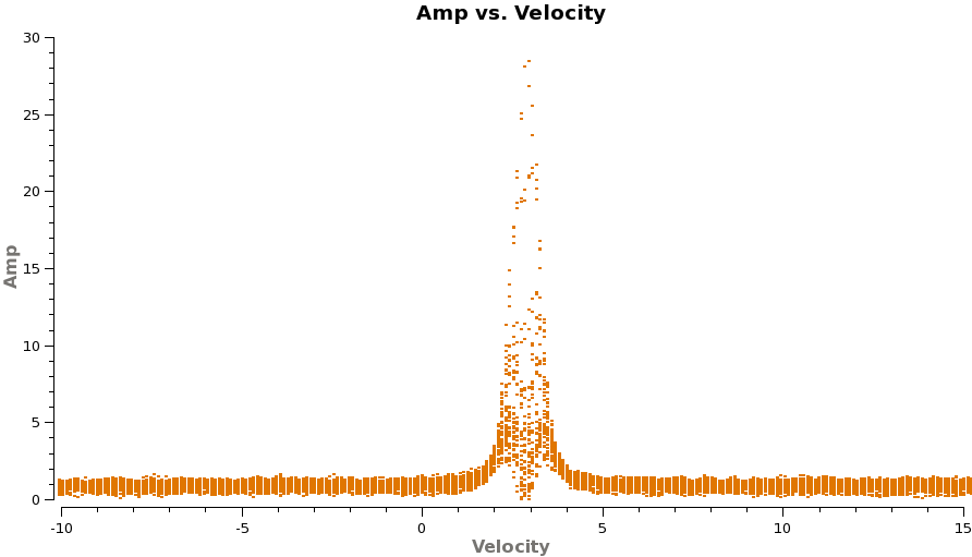
# In CASA
for asdm in basename:
  plotms(vis='Band7multi_april22.ms',spw='2',xaxis='velocity',yaxis='amp',field='2',
         avgtime='1e8',avgscan=T,transform=T,freqframe='LSRK',restfreq='345.79599GHz',
         plotrange=[-10,15,0,0],coloraxis='spw')
  print('When you are done with the graphics window,')
  print('quit that window, and')
  user_check=raw_input('press enter to continue script\n')
Fix Titan's Coordinates
Note that in the near future this step will be unnecessary.
It is temporarily necessary to correct the positions of ephemeris objects observed by ALMA, as they are currently erroneously written to the data with coordinates of 00:00:00.0000 +00.00.00.0000 J2000 (see listobs output in TWHydraBand7_Calibration#Observing_Log_and_Priors). For this data we need to correct Titan which we observed as the absolute flux calibrator. It is important to apply the fix after concatenation of the data, or Titan will be at slightly different positions in all three datasets.
If you are running casa revision r15777 or newer, fixplanets() is already defined as a task. However, if you are using an older revision, then you must first initialize this script with this command:
execfile(casadef.python_library_directory+'/recipes/fixplanets.py')
Now fix the position of Titan. This step takes a while because the model and corrected scratch columns must be created for the new dataset first (see logger message).
# In CASA
fixplanets(vis='Band7multi_april22.ms', field='Titan', fixuvw=True)
Check the header information again to see that the information for Titan has changed.
# In CASA
listobs(vis='Band7multi_april22.ms',verbose=F)
  ID   Code Name         RA            Decl           Epoch   SrcId
  0    none 3c279        12:56:11.1666 -05.47.21.5247 J2000   0
  1    none Titan        12:49:26.5120 -02.22.10.8190 J2000   1
  2    none TW Hya       11:01:51.9063 -34.42.17.0212 J2000   2
  3    none J1147-382=Q* 11:47:01.3815 -38.12.11.1179 J2000   3
  4    none J1037-295=Q* 10:37:16.0899 -29.34.02.9888 J2000   4
Split Calibrated Data
Now we split off the calibrated data for the Science Target as well as the interesting parts of the calibrators for imaging.
# In CASA
os.system('rm -rf TWHydra_corrected.ms')
split(vis='Band7multi_april22.ms',outputvis='TWHydra_corrected.ms',
      datacolumn='corrected',spw='',field='2')
# In CASA
os.system('rm -rf J1037_corrected.ms')
split(vis='Band7multi_april22.ms',outputvis='J1037_corrected.ms',
      datacolumn='corrected',spw='',field='4')
# In CASA
os.system('rm -rf J1147_corrected.ms')
split(vis='Band7multi_april22.ms',outputvis='J1147_corrected.ms',
      datacolumn='corrected',spw='',field='3')
# In CASA
os.system('rm -rf J1147_corrected_with4.ms')
split(vis='Band7multi_april22.ms',outputvis='J1147_corrected_with4.ms',
      datacolumn='corrected',spw='',field='3')
# In CASA
os.system('rm -rf Titan_cont.ms')
split(vis='Band7multi_april22.ms',outputvis='Titan_cont.ms',
      datacolumn='corrected',spw='0',field='1')
# In CASA
os.system('rm -rf Titan_CO3_2.ms')
split(vis='Band7multi_april22.ms',outputvis='Titan_CO3_2.ms',
      datacolumn='corrected',spw='2',field='1')
# In CASA
os.system('rm -rf Titan_unknown.ms')
split(vis='Band7multi_april22.ms',outputvis='Titan_unknown.ms',
      datacolumn='corrected',spw='3',field='1')
# In CASA
os.system('rm -rf 3C279_CO3_2.ms')
split(vis='Band7multi_april22.ms',outputvis='3C279_CO3_2.ms',
      datacolumn='corrected',spw='2:1900~2000',field='0')
Imaging Calibrators
This section will be added soon.
Continue on to Imaging of the Science Target
Now you can continue on to the imaging guide.
Last checked on CASA Version 3.3.0.

