VLA Radio galaxy 3C 129: P-band continuum tutorial-CASA6.4.1
This CASA Guide is for Version 6.4.1 of CASA.
Note: This guide may take up to 2 days to complete
If you are using a later version of CASA and this is the most recent available guide, then you should be able to use most, if not all, of this casaguide, as we try to limit script breaking changes in CASA development.
Overview
This webpage provides a basic description on how to use CASA to reduce data from the upper part of the new VLA low-band system, also known as P-band, covering 200-500 MHz (the default setup and recommended usable band is 224-480 MHz). The goal is to make a wide-field continuum stokes I image of a typical blank field using the full effective bandwidth. The dataset that will be downloaded in this guide has a size of 26.46 GB and will require a total of ~140 GB of disk space if all generated files are kept.
Note: CASA 6.2.0 uses IPython 7.15.0 for interactive CASA sessions. This does not allow to readily paste and execute multiple lines of code like in previous versions of the interpreter. If this is needed at any point in this tutorial, we use "%cpaste" to allow the copy/paste of loops, conditions, etc.. Press "Enter" (or "Return") after "--" at the end, this stops (or exits) the copy/paste prompt and will return you to the CASA prompt.
Obtaining the raw data
For this guide, we'll use some test data that was taken in B-configuration. To get a copy of the raw data, download P_band_3C129.tgz onto your computer running CASA and untar it (i.e. tar -zxvf <filename>).
Alternatively, the raw data can also be obtained from the NRAO archive, go to the NRAO advance archive query page, and enter the following search parameter in the search field (leave the rest on default):
imag-test-copy.57080.956837025464
The search should return a single row for Archive File: imag-test-copy.57080.956837025464, taken on Feb. 27, 2015 (or "15-Feb-27 22:57:52"). Check the box next to it. Next, fill in your email and select the "SDM-BDF dataset (all files)" option. Note, you may find it easier to download a tar file, in which case, you'll want to check the box for Create MS or SDM tar file. Click "Get My Data" and follow the on-screen prompts to reach the next page, where you should click "Retrieve over internet". The next page should report that the data staging is in progress. Wait until you receive an e-mail reporting that your archive data is copied, which should take a few minutes. Download the data onto your computer running CASA and untar it (i.e. tar -xvf <filename>).
Starting CASA
Start CASA by typing
casa -r 6.4.1-12-pipeline-2022.2.0.64
on the (linux) command line. This should start a CASA 6.2.0 interactive python (iPython) session, and open a separate log window. The CASA version is reported at startup, both in the python session and the log window.
Importing the raw data into CASA
We will begin by importing our data into the measurement set format (CASA standard) from the binary format (SDM-BDF) as downloaded from the archive. We do this by means of the importasdm task. It is important to note that the importevla task has been deprecated.
# In CASA
importasdm(asdm='imag-test-copy.57080.956837025464', vis='3C129.ms', savecmds=True, outfile='importflags.txt')
This task calls the external tool asdm2MS to perform the conversion. Together with the visibility data, also the flag commands from the VLA online system are imported. These flags are not directly applied, but stored in the importflags.txt file and applied later.
Preliminary data inspection
Inspect the observation setup with the listobs task, which now returns a dictionary that contains some of the fundamental listobs output. Setting a variable when calling listobs prevents these dictionary values from printing to terminal. The following command will save the output to a file.
# In CASA
listobs_file = listobs(vis='3C129.ms', verbose=True, listfile='3C129.listobs')
Alternatively, you can also output to the logger by running the command without the listfile argument. The sample listobs output shown has flag verbose=False for the sake of brevity.
# In CASA
listobs_logger = listobs(vis='3C129.ms', verbose=False)
================================================================================
           MeasurementSet Name:  /lustre/aoc/sciops/fschinze/P_band_tutorial/3C129.ms      MS Version 2
================================================================================
   Observer:      Project: uid://evla/sdm/X2
Observation: EVLA(27 antennas)
Data records: 4714983       Total elapsed time = 1422 seconds
   Observed from   27-Feb-2015/22:57:54.0   to   27-Feb-2015/23:21:36.0 (UTC)

Fields: 2
  ID   Code Name                RA               Decl           Epoch   SrcId      nRows
  0    NONE 3C147               05:42:36.127300 +49.51.07.17800 J2000   0        1307124
  1    NONE 3C129               04:48:58.200000 +45.02.01.00000 J2000   1        3407859
Spectral Windows:  (19 unique spectral windows and 1 unique polarization setups)
  SpwID  Name           #Chans   Frame   Ch0(MHz)  ChanWid(kHz)  TotBW(kHz) CtrFreq(MHz) BBC Num  Corrs
  0      EVLA_P#A0C0#0     128   TOPO     224.000       125.000     16000.0    231.9375       12  XX  XY  YX  YY
  1      EVLA_P#A0C0#1     128   TOPO     240.000       125.000     16000.0    247.9375       12  XX  XY  YX  YY
  2      EVLA_P#A0C0#2     128   TOPO     256.000       125.000     16000.0    263.9375       12  XX  XY  YX  YY
  3      EVLA_P#A0C0#3     128   TOPO     272.000       125.000     16000.0    279.9375       12  XX  XY  YX  YY
  4      EVLA_P#A0C0#4     128   TOPO     288.000       125.000     16000.0    295.9375       12  XX  XY  YX  YY
  5      EVLA_P#A0C0#5     128   TOPO     304.000       125.000     16000.0    311.9375       12  XX  XY  YX  YY
  6      EVLA_P#A0C0#6     128   TOPO     320.000       125.000     16000.0    327.9375       12  XX  XY  YX  YY
  7      EVLA_P#A0C0#7     128   TOPO     336.000       125.000     16000.0    343.9375       12  XX  XY  YX  YY
  8      EVLA_P#A0C0#8     128   TOPO     352.000       125.000     16000.0    359.9375       12  XX  XY  YX  YY
  9      EVLA_P#A0C0#9     128   TOPO     368.000       125.000     16000.0    375.9375       12  XX  XY  YX  YY
  10     EVLA_P#A0C0#10    128   TOPO     384.000       125.000     16000.0    391.9375       12  XX  XY  YX  YY
  11     EVLA_P#A0C0#11    128   TOPO     400.000       125.000     16000.0    407.9375       12  XX  XY  YX  YY
  12     EVLA_P#A0C0#12    128   TOPO     416.000       125.000     16000.0    423.9375       12  XX  XY  YX  YY
  13     EVLA_P#A0C0#13    128   TOPO     432.000       125.000     16000.0    439.9375       12  XX  XY  YX  YY
  14     EVLA_P#A0C0#14    128   TOPO     448.000       125.000     16000.0    455.9375       12  XX  XY  YX  YY
  15     EVLA_P#A0C0#15    128   TOPO     464.000       125.000     16000.0    471.9375       12  XX  XY  YX  YY
  16     EVLA_P#B0D0#16     64   TOPO     310.000       500.000     32000.0    325.7500       15  XX  XY  YX  YY
  17     EVLA_P#B0D0#17   1024   TOPO     310.000        62.500     64000.0    341.9688       15  XX  XY  YX  YY
  18     EVLA_P#B0D0#18     64   TOPO     342.000       500.000     32000.0    357.7500       15  XX  XY  YX  YY
Antennas: 27 'name'='station'
   ID=   0-3: 'ea01'='N12', 'ea02'='N16', 'ea03'='W28', 'ea05'='E20',
   ID=   4-7: 'ea06'='N20', 'ea07'='N32', 'ea08'='E28', 'ea09'='W08',
   ID=  8-11: 'ea10'='E36', 'ea11'='W12', 'ea12'='N36', 'ea13'='W04',
   ID= 12-15: 'ea14'='E08', 'ea15'='E24', 'ea16'='W24', 'ea17'='E04',
   ID= 16-19: 'ea18'='W36', 'ea19'='MAS', 'ea20'='N04', 'ea21'='E32',
   ID= 20-23: 'ea22'='N24', 'ea23'='E16', 'ea24'='W32', 'ea25'='W20',
   ID= 24-26: 'ea26'='E12', 'ea27'='N08', 'ea28'='N28'
You can inspect the output text file 3C129.listobs in your favorite text editor (e.g., gedit). When taking some time to familiarize yourself with the output format, you will see that:
- The observation consists of 5 scans, namely:
- 3C147 (hardware setup)
- 3C147 (setting requantizers)
- 3C147 (primary calibrator)
- 3C129 (target)
- 3C129 (target)
- The frequency coverage is 224 - 480 MHz, divided into 16 x 16 MHz spectral windows, each having 128 x 0.125 MHz channels. There are also two spectral windows with 64x0.5 MHz and one spectral window with 1024x0.0625 MHz.
- Visibilities are recorded every 2 seconds in full polarization (4 polarization products labelled XX,XY,YX,YY).
- Of the 28 VLA antennas labelled ea01 - ea28, antenna ea04 is not participating in this observation.
- Source, antenna and spectral window IDs start at zero, but scan IDs start at one.
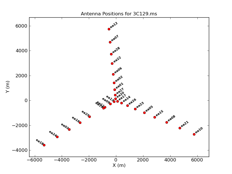
The array configuration can be inspected using plotants:
# In CASA
plotants(vis='3C129.ms', figfile='3C129_pband_plotants.png')
Initial processing steps - Hanning smoothing, Antenna Position, Requantizer Gain, Ionospheric Correction
Initial data editing
When importing the data, we saved the flags from the online system to an ASCII text file. This gives us the opportunity to review the flag commands before applying them. For our data set, the flag file is called importflags.txt. Open this file with your favorite text editor. The bulk of the flag commands refer to times when the VLA is slewing (ANTENNA_NOT_ON_SOURCE) or when the movable secondary reflector of the VLA's Cassegrain system is not in place (SUBREFLECTOR_ERROR). The latter can cause antenna gain variations (amplitude and phase), so it is safest to apply all the flags. In order to remove visibilities that are pure zero, and flag antennas that are partly blocked by other antennas (shadowing), which occurs mostly in compact configurations when observing at low elevation along a VLA arm, two lines need to be appended to importflags.txt. These are:
mode='clip' clipzeros=True
mode='shadow' tolerance=0.0
After this, execute flagdata in CASA:
# In CASA
flagdata(vis='3C129.ms', mode='list', inpfile='importflags.txt', action='apply', reason='any', flagbackup=True)
This call, before applying the new flags to the data, created a new flagbackup file called flagdata_1 which can be used by the task flagmanager to restore the state of the measurement set prior to applying the flags from importflags.txt.
Dead antennas
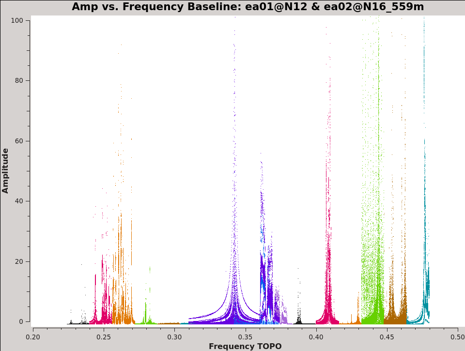
It is important to identify dead antennas / polarizations early on, so we can exclude them from further data processing. A convenient way of doing this is through the plotms task on bright calibrator(s) (see the listobs output), in our case 3C147 (see Fig. 2a).
# In CASA
plotms(vis='3C129.ms',xaxis='freq',yaxis='amp',antenna='ea01',correlation='XX,YY', field='3C147',
           plotrange=[0.2,0.5,0.0,100.0], coloraxis='spw',xlabel='Frequency',ylabel='Amplitude',iteraxis='baseline',
           plotfile='3C129_pband_3C147_prebp.png')
This will load the plotms window that will iterate over all the baselines to antenna ea01. (Note: when running plotms with both iteraxis and plotfile, casa will write the first iteration plotted by plotms to the .png, and append the file name to specify this. For example, the png file here will be named 3C129_pband_3C147_prebp_Baselineea01@N12_with_ea02@N16_559m.png). The plot will display amplitude vs frequency with the colors representing the different spectral windows. Note that we are only plotting the XX and YY correlation here. This is because we expect most of the power in the linear cross correlation products to be in these two correlations. Notice that some spectral windows in particular are badly affected due to radio frequency interference (RFI). We will deal with this issue after identifying dead antennas. If you page through the baselines using the green forward button in the plotms viewer, you will notice that the amplitude is particularly low when you encounter ea19. If we create a quick plot of the baselines to ea19 (put ea19 in the antenna field), we can see that there is no power in any of the polarizations. This indicates that this antenna was dead and should be flagged. It is also good to check for high power levels in cross-hand correlations in comparison to the parallel-hand correlations, which would uncover swapped polarization labels and severely mis-aligned dipoles. At the end of this tutorial we provide some hints on solving for swapped or mislabeled dipole polarizations. In addition to the dead antenna, we also make sure that the first two scans are flagged, which were not labelled as setup scans but were used to set the attenuators and requantizers during the observation.
# In CASA
flagdata(vis='3C129.ms',mode='manual',antenna='ea19')
#
flagdata(vis='3C129.ms',mode='manual',scan='1~2')
Hanning smoothing
During the data inspection above, we also notice sharp RFI peaks. Often this is due to Gibbs ringing (Gibbs phenomenon), and to prevent this phenomenon it is best to Hanning smooth the data at this juncture. The default P-band setup contains 16x16 MHz spectral windows. For Hanning smoothing we will select the first 16 spectral windows. Note that the task hanningsmooth will create a new MS. This will also make the hanning smoothed dataset smaller and faster to process. Now is a good time to get a cup of coffee while the task is hanning smoothing the data.

# In CASA
hanningsmooth(vis='3C129.ms',outputvis='3C129_pband.ms',datacolumn='data',spw='0~15')
Once the task is finished we should replot the primary calibrator to see the effect of hanning smoothing on the data and the RFI (Fig. 2b).
# In CASA
plotms(vis='3C129_pband.ms',xaxis='freq',yaxis='amp',antenna='ea01',correlation='XX,YY',
           field='3C147', plotrange=[0.2,0.5,0.0,100.0], coloraxis='spw',xlabel='Frequency',ylabel='Amplitude',
           iteraxis='baseline', plotfile='3C129_pband_3C147_prebp_hanning.png')
Antenna Position Corrections
It is always a good idea to check if the antenna position offsets need corrections. Antenna positional errors translate to an error in the measured visibilities and, if present, they need to be accounted for before we proceed with any of the other calibration steps. We use the task gencal. Note that caltype='antpos' requires internet connection to access the VLA antenna position correction site.
# In CASA
gencal(vis='3C129_pband.ms',caltable='3C129_pband.antpos',caltype='antpos')
The logger output shows that there are 13 antennas with positional offsets:
2016-11-28 22:51:37 INFO gencal	offsets for antenna ea03 :  0.00290   0.00000   0.00000
2016-11-28 22:51:37 INFO gencal	offsets for antenna ea08 :  0.00000   0.00390   0.00000
2016-11-28 22:51:37 INFO gencal	offsets for antenna ea10 : -0.00170   0.00000   0.00400
2016-11-28 22:51:37 INFO gencal	offsets for antenna ea11 :  0.00000   0.00160  -0.00170
2016-11-28 22:51:37 INFO gencal	offsets for antenna ea13 :  0.00000   0.00050   0.00000
2016-11-28 22:51:37 INFO gencal	offsets for antenna ea16 : -0.00180   0.00680   0.00230
2016-11-28 22:51:37 INFO gencal	offsets for antenna ea18 :  0.00470   0.00350   0.00000
2016-11-28 22:51:37 INFO gencal	offsets for antenna ea21 : -0.00160   0.00000   0.00210
2016-11-28 22:51:37 INFO gencal	offsets for antenna ea23 :  0.00140   0.00200  -0.00150
2016-11-28 22:51:37 INFO gencal	offsets for antenna ea24 :  0.00380   0.00000  -0.00340
2016-11-28 22:51:37 INFO gencal	offsets for antenna ea25 :  0.00330   0.00000  -0.00110
2016-11-28 22:51:37 INFO gencal	offsets for antenna ea26 :  0.00000   0.00190   0.00000
2016-11-28 22:51:37 INFO gencal	offsets for antenna ea27 : -0.00120   0.00070   0.00000
Ionospheric TEC Corrections
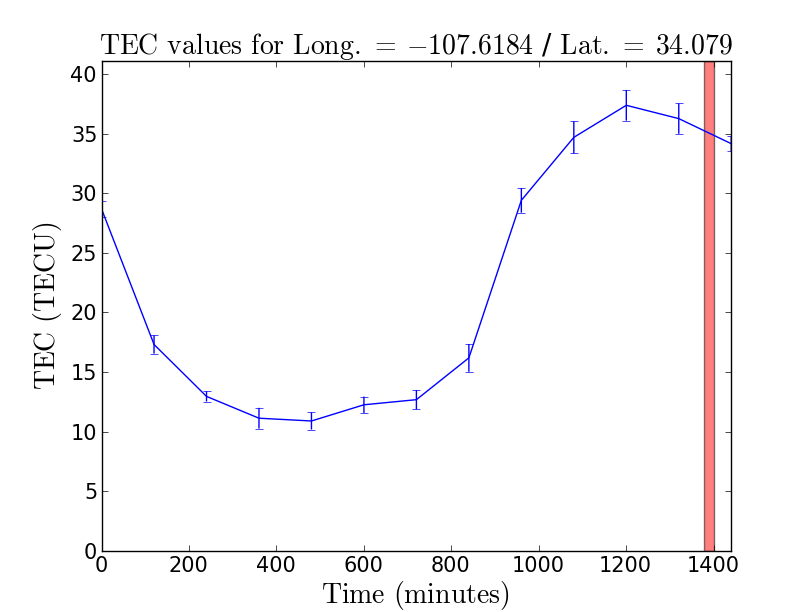
Low frequency observations are affected by the ionosphere. A delay in the signal path is introduced between the two polarizations of light that varies both as a function of time and line of sight (direction dependent). The delay is proportional to the Total Electron Content (TEC) along the line of sight (∝TEC), and is inversely proportional to the square of the frequency (∝1/ν^2). GPS measurements at two different frequencies provide us with an estimate of the TEC per square meter. This correction has been implemented in CASA which we shall apply as a calibration table with the gencal task. The task requires a TEC map that we will generate with CASA recipes and can be viewed with CARTA. For more information, see the section on ionospheric corrections in the CASA docs. For some versions of CASA, the first plot to the right (Figure 3) may not be generated if you have already run plotants: to generate this plot, you will need to restart CASA. If the IONEX data file was not downloaded, you might be missing the curl package in the environment you are running CASA in. In such a case you can provide the required file manually by downloading: ftp://cddis.gsfc.nasa.gov/gnss/products/ionex/2015/058/igsg0580.15i.Z (for the tutorial it is also also available in an unzipped version here), unzipping it, and placing it in the directory from which you started CASA. The current implementation in CASA is in the development stage, however since the CASA 5.0 release both the Faraday rotation correction and dispersive delay corrections for the ionosphere are enabled. In previous releases only Faraday rotation corrections are enabled. In this example we will generate the calibration table and apply it throughout calibration.
# In CASA
#
from casatasks.private import tec_maps
# CASA 5 or earlier: from recipes import tec_maps
#
tec_image, tec_rms_image, plotname = tec_maps.create(vis='3C129_pband.ms',doplot=True)
# CASA 5.0.0 or earlier: tec_image, tec_rms_image = tec_maps.create(vis='3C129_pband.ms', doplot=True)
#
gencal(vis='3C129_pband.ms',caltable='3C129_pband.tecim',caltype='tecim',infile=tec_image)
#
# Spatial plots like shown in Figure 4 can be looked at using the CARTA viewer for the TEC values
carta 3C129_pband.ms.IGS_TEC.im
#
# and for TEC rms
carta 3C129_pband.ms.IGS_RMS_TEC.im
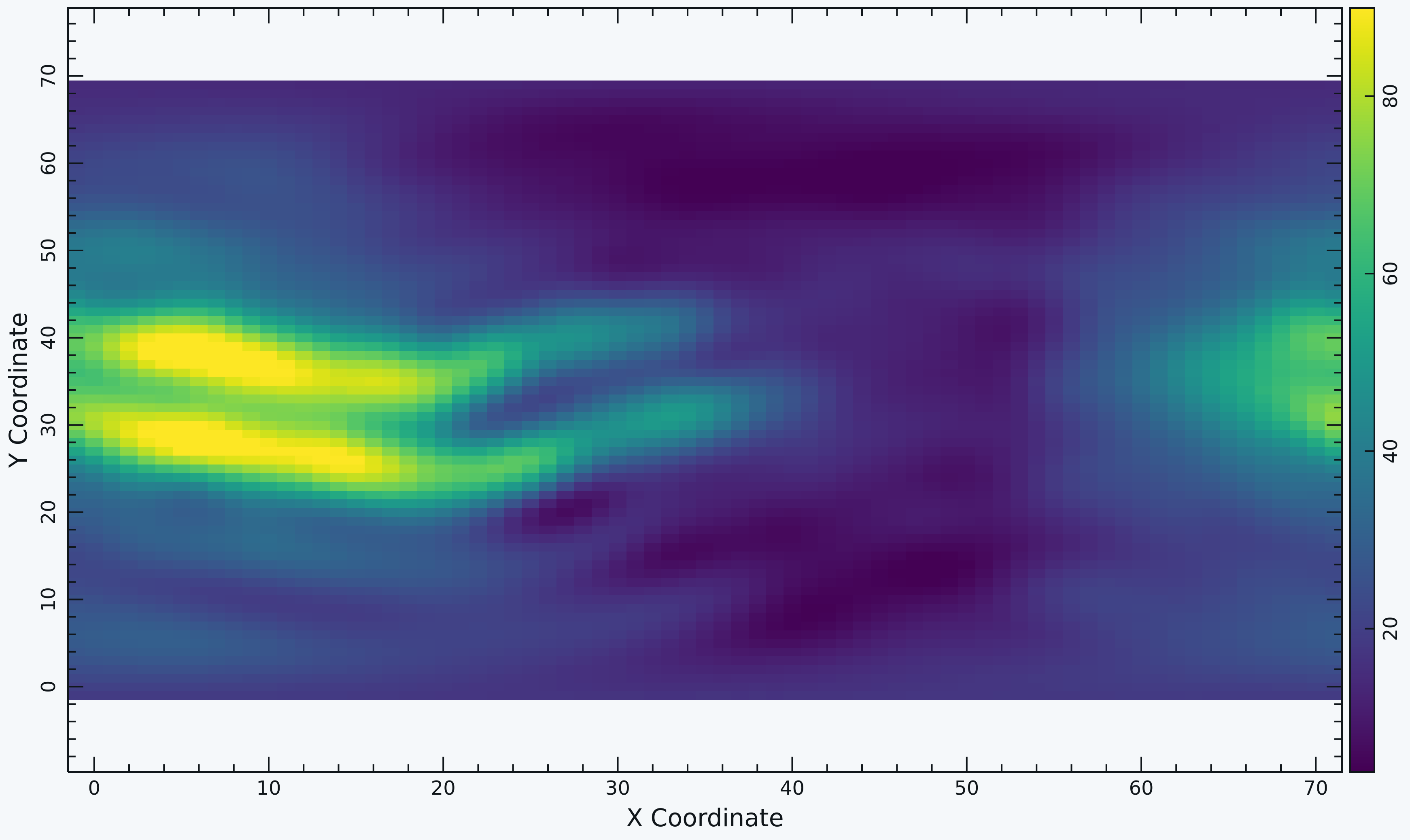
A word of caution regarding the TEC map generation: the IGS website updates measurements only two weeks after the date of observation.
Requantizer Gains
The next step will correct the visibility amplitudes for the signal leveling (requantizer gains) that occurs at the inputs of the WIDAR correlator. These levels (per antenna, per polarization, per spectral window) are stored with the measurement set (in the SYSPOWER sub-table). This step is currently not essential, since the levels get set only once at the start of an observation and bandpass calibration will correct for this, but it will make your bandpass plots look better if you have multiple spectral windows. More importantly, it is possible to trigger the setting of requantizers throughout an observation. This is the case for new observations, when a P-band scan is preceded by a P-band setup scan, which itself is preceded by a scan with a different telescope configuration.
The correction is done by means of the gencal task, where information in the SYSPOWER sub-table gets translated into a gain table.
# In CASA
gencal(vis='3C129_pband.ms',caltype='rq',caltable='3C129_pband.rq')
Automatic flagging
It is worthwhile noting at this juncture that the standard P-band setup will ensure that the worst of the RFI is restricted to four of the spectral windows. This particular dataset is an example of higher than average levels of RFI across the band. Before throwing away bad spectral windows by hand, we'll let the automated flaggers in CASA have a go at it. The main task for this is flagdata. While working on your data, flagdata produces an abundance of output, not all of which is easy to understand. To help with this, we can get the flag status of our data before and after auto-flagging by running flagdata in the summary mode. This first call provides the flag statistics of the flagging up to now, before any auto-flagging:
summary_1 = flagdata(vis='3C129_pband.ms', mode='summary')
This returns a python dictionary with flagged versus total visibilities along various axes (antenna, scan, spw, field, correlation, etc.). For example, if we want to know the percentage flagged per scan, run the following (note that the scans may not appear in sorted order):
# In CASA
%cpaste

# Press Enter or Return, then copy/paste the following:
axis = 'scan'
for id, stats in summary_1[ axis ].items():
  print('%s %s: %5.1f percent flagged' % ( axis, id, 100. * stats[ 'flagged' ] / stats[ 'total' ] ))
--
For this example, you will notice that scans 1 and 2 (the dummy scans on 3C147) are 100 percent flagged, which is what we did during the initial flagging.
We will run flagdata in the tfcrop mode, which will (per scan, per baseline, per spectral window, per polarization) look for visibility amplitude outliers. It uses a 5-piece polynomial in an attempt to remove any intrinsic bandpass (amplitude) structure (we did not calibrate for bandpass yet). We run the task twice to allow for slightly deeper flagging and separate treatment of the parallel and cross-hand correlations. For the first run, we tell CASA to make a backup of our visibility flag status up to here, giving us an option to restore them if we choose over-aggressive flagging parameters and consequently over-flag our data. The flag backup file name is reported in the log window, and can be found in the 3C129_pband.ms.flagversions directory.
# In CASA
flagdata(vis='3C129_pband.ms', field='*', mode='tfcrop', datacolumn='data', timecutoff=4., freqcutoff=3., maxnpieces=5,
  action='apply', display='report', flagbackup=True, combinescans=True, ntime='3600s', correlation='ABS_XY,ABS_YX')
#
flagdata(vis='3C129_pband.ms', field='*', mode='tfcrop', datacolumn='data', timecutoff=3., freqcutoff=3., maxnpieces=2,
  action='apply', display='report', flagbackup=False, combinescans=True, ntime='3600s', correlation='ABS_XX,ABS_YY')
#
flagdata(vis='3C129_pband.ms', mode='extend')
As a note of caution: When executing flagdata with mode='extend', all flags that were ever applied to the dataset will get extended. Repeat execution of this command will incrementally flag more and more around already flagged data.
Let's get another flag summary to see how much extra data was flagged:
# In CASA
summary_2 = flagdata(vis='3C129_pband.ms' , mode='summary')
#
%cpaste

# Press Enter or Return, then copy/paste the following:
axis = 'scan'
for value, stats in summary_2[ axis ].items():
  old_stats = summary_1[ axis ][ value ]
  print('%s %s: %5.1f percent flagged additionally' % ( axis, value, 100. * ( stats[ 'flagged' ] - old_stats[ 'flagged' ] ) / stats[ 'total' ] ))
--
#
plotms(vis='3C129_pband.ms',xaxis='freq',yaxis='amp',antenna='ea01',correlation='XX,YY',
           field='3C147', plotrange=[0.2,0.5,0.0,100.0], coloraxis='spw',xlabel='Frequency',ylabel='Amplitude',
           iteraxis='baseline', plotfile='3C129_pband_3C147_prebp_hanning_automatic.png')
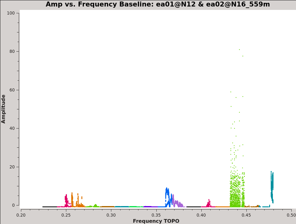
There is quite a bit of RFI that gets missed in RFI-rich spectral windows as can be seen in Fig. 5a. The solution to this is to provide the flagging routines with more contrast between healthy and affected data. For this, we will perform a preliminary bandpass calibration to take out the bandpass shape. We will do some coarse preliminary calibration and apply it to the calibrator before flagging for RFI once more. Tasks gaincal, bandpass, and applycal are used.
# In CASA
gaincal(vis='3C129_pband.ms', caltable='3C129_pband.G0', gaintype='G', calmode='p', solint='int', field='3C147',refant='ea09',
  gaintable=['3C129_pband.antpos','3C129_pband.rq','3C129_pband.tecim'])
#
gaincal(vis='3C129_pband.ms', caltable='3C129_pband.K0', gaintype='K', solint='inf', field='3C147',refant='ea09',
  gaintable=['3C129_pband.antpos','3C129_pband.rq','3C129_pband.tecim','3C129_pband.G0'])
#
bandpass(vis='3C129_pband.ms', caltable='3C129_pband.B0', solint='inf', field='3C147',refant='ea09', minsnr=2.0,
  gaintable=['3C129_pband.antpos','3C129_pband.rq','3C129_pband.tecim','3C129_pband.G0','3C129_pband.K0'])
#
applycal(vis='3C129_pband.ms', field='3C147', applymode='calflagstrict',
  gaintable=['3C129_pband.antpos','3C129_pband.rq','3C129_pband.tecim','3C129_pband.G0','3C129_pband.K0','3C129_pband.B0'] )
On the command line you should see a notification stating: "FJones (iononsphere) apply now provisionally includes disp. delay." which indicates that both Faraday rotation as well as dispersive delay corrections for the ionosphere are applied.

We will now flag the corrected data column that contains the coarsely calibrated visibilities which provide better contrast to the flagging algorithms to remove the RFI present. We will begin by running the rflag algorithm in the task flagdata. We will again use summary mode to see how much more of the observed data was flagged.
# In CASA
flagdata(vis='3C129_pband.ms', field='3C147', mode='rflag', datacolumn='corrected', timedevscale=4., freqdevscale=3.,
  action='apply',  flagbackup=True, combinescans=True, ntime='3600s')
#
summary_3 = flagdata(vis='3C129_pband.ms', mode='summary')
#
%cpaste
# Press Enter or Return, then copy/paste the following:
axis = 'scan'
for value, stats in summary_3[ axis ].items():
  old_stats = summary_2[ axis ][ value ]
  print('%s %s: %5.1f percent flagged additionally' % ( axis, value, 100. * ( stats[ 'flagged' ] - old_stats[ 'flagged' ] ) / stats[ 'total' ] ))
--
#
plotms(vis='3C129_pband.ms',xaxis='freq',yaxis='amp',antenna='ea01',correlation='XX,YY',
           field='3C147', plotrange=[0.2,0.5,0.0,100.0], coloraxis='spw',xlabel='Frequency',ylabel='Amplitude',
           iteraxis='baseline', plotfile='3C147_postbandpass_rflag.png', ydatacolumn='corrected')
Taking another visual look at the data using plotms, we examine the effect of the automated flagging on the calibrator (Fig. 5b). We find that most spectral windows are RFI free and that about 37% of the data was flagged. We typically expect between 40-60% of flagging due to interference in a significant fraction of the band. In this example, a more careful RFI flagging approach is likely to recover more usable spectrum.
Absolute Flux Density Calibration
Our flagging has cleaned up most of the stray RFI across the band. This allows us to proceed with the actual calibration of the data. Before we get to the calibration tables, it's essential to do the flux density calibration of our calibrator 3C147. This is done by the setjy task. Before we run the task we first clear the preliminary calibration that was carried out to enable better flagging. We do that by running the clearcal task.
# In CASA
clearcal(vis='3C129_pband.ms')
# In CASA
setjy(vis='3C129_pband.ms', field='3C147', standard='Scaife-Heald 2012', usescratch=True)
The default Perley-Butler 2017 standard has a P band model for 3C147 as well.
Delay and bandpass calibration
First, we use the full bandwidth on a single scan on the primary calibrator to determine a single delay per antenna, per polarization. This will determine a single (approximate) phase slope across frequency, mainly caused by propagation effects in the (time-variable) ionosphere, cable length differences, and electronics in the signal paths from antenna feeds to correlator. Note that for a single short (5-10 minutes) scan on the calibrator, we can get away with solving for a time-invariant delay per antenna, per polarization. We will use scan 3 on 3C147.

# In CASA
gaincal(vis='3C129_pband.ms', caltable='3C129_pband.K1', field='3C147', solint='inf', refant='ea09', gaintype='K',
   gaintable=['3C129_pband.antpos','3C129_pband.tecim','3C129_pband.rq'],parang=True)
#
plotms(vis='3C129_pband.K1',xaxis='antenna1',yaxis='delay',plotrange=[0,30,-50.,50.])
Since we picked ea09 as our reference antenna, the delays for this antenna ID are arbitrarily set to zero. All other delays should be within 30 nanosec or so (which they should be for this data set; Fig. 6). Larger values, which you can see if you do not force the plotrange, should be treated with suspicion, indicating a problem with the antenna or polarization. We will use the bandpass calibration to verify this in the next step.
To determine the bandpass calibration, we use the same source and scan and apply the delay calibration before solving for the bandpass. Note that we request a minimum SNR of 3, which will make the solve fail for the worst, but not all, channels.
# In CASA
bandpass(vis='3C129_pband.ms', caltable='3C129_pband.B1', field='3C147', solint='inf', refant='ea09', minsnr=3.0,
                parang = True, gaintable=['3C129_pband.antpos','3C129_pband.tecim','3C129_pband.rq','3C129_pband.K1'],
                interp=['','','','nearest,nearestflag'])
After solving, we inspect the bandpass calibration amplitudes and phase, and flag any obvious residual outliers. Outliers may be found above or below the average bandpass curves, and tend to arise in the same channel (frequency) ranges for all antennas.
# In CASA
plotms(vis='3C129_pband.B1', xaxis='freq', yaxis='amp', iteraxis='antenna', coloraxis='spw')
#
plotms(vis='3C129_pband.B1', xaxis='freq', yaxis='phase', iteraxis='antenna', plotrange=[0,0,-180.,180.], coloraxis='spw')
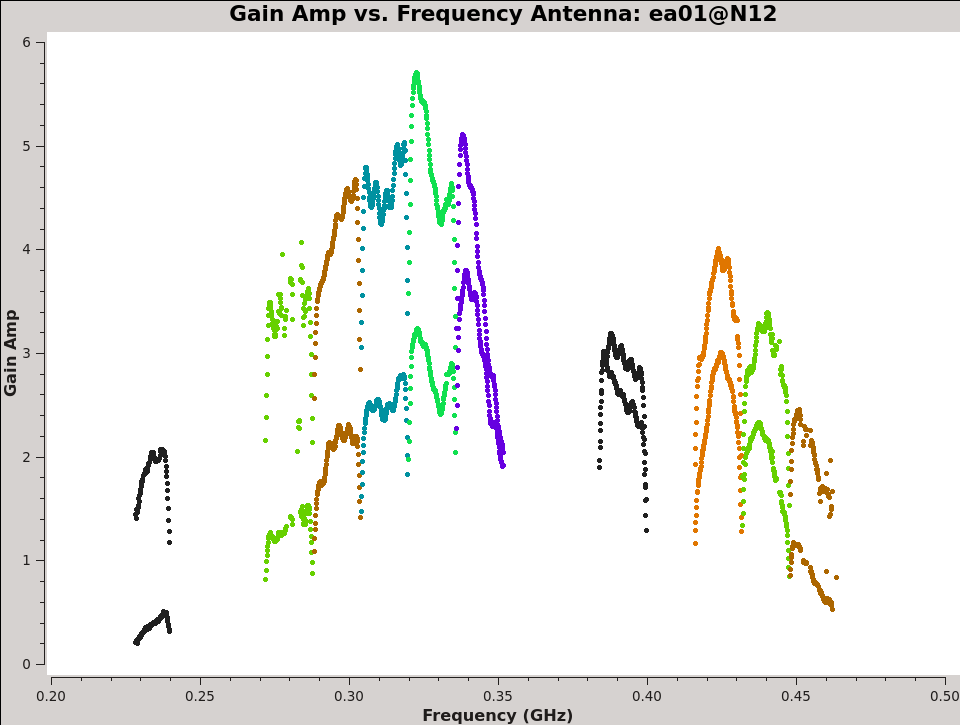
Note that the bandpass amplitudes (Fig. 7a) and phases (Fig. 7b) may differ between polarizations of the same antenna. The bandpass phases across frequency should not have an overall gradient (this should be removed by the delay calibration), but they may wrap around from +/-180 to -/+180 degrees. If that is problematic, re-run the phase plotms with plotrange = [ .2,.5,0.,360. ]. Also note that there are no bandpass solutions for antennas ea19 and ea28, and only a few solutions for ea14.
Don't spend more than 1 minute per antenna to find and flag the outliers in this tutorial and don't worry about missing some bad points; these bad channels will likely get flagged in a later stage anyway. We don't set the scale for plotting the bandpass amplitudes, which is convenient when flagging outliers as it will auto-rescale. While plotting the bandpass phases we do fix the scale, as it provides a better feeling for the relevant magnitude of phase outliers. Flagging of outliers is done using the Mark Region and Flag buttons. For more information on interactive flagging, see the topical guide Flagging VLA Data in CASA. We are using this mechanism to efficiently flag data manually, since it is done per antenna rather than per baseline. These 'flags' will not be permanent until we call applycal later on, but are effective while applying the calibration on the fly, as we will do in subsequent calibration steps.
 |
 |
Gain calibration
With the delay and bandpass calibration in place, we will now look more closely at the time-variable behavior of the VLA. We use the same scan on our primary calibrator, 3C147, over the full effective bandwidth to determine gain calibrations: one complex value per antenna, per polarization, per integration time. The delay and bandpass tables are applied on the fly.
# In CASA
gaincal(vis='3C129_pband.ms', caltable='3C129_pband.G1', field='3C147', solint='int',
             refant='ea09', minsnr=3.0, gaintype='G', calmode='ap',
             gaintable=['3C129_pband.antpos','3C129_pband.rq','3C129_pband.tecim','3C129_pband.K1','3C129_pband.B1'],
             interp=['','','','nearest,nearestflag','nearest,nearestflag'], parang=True)
Again, the solutions should be inspected for any outliers.
# In CASA
plotms(vis='3C129_pband.G1', xaxis='time', yaxis='amp', iteraxis='antenna', coloraxis='spw')
#
plotms(vis='3C129_pband.G1', xaxis='time', yaxis='phase', plotrange=[0,0,-180.,180.], iteraxis='antenna', coloraxis='spw')
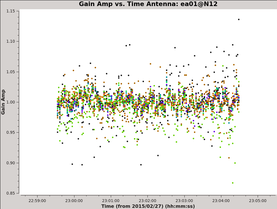
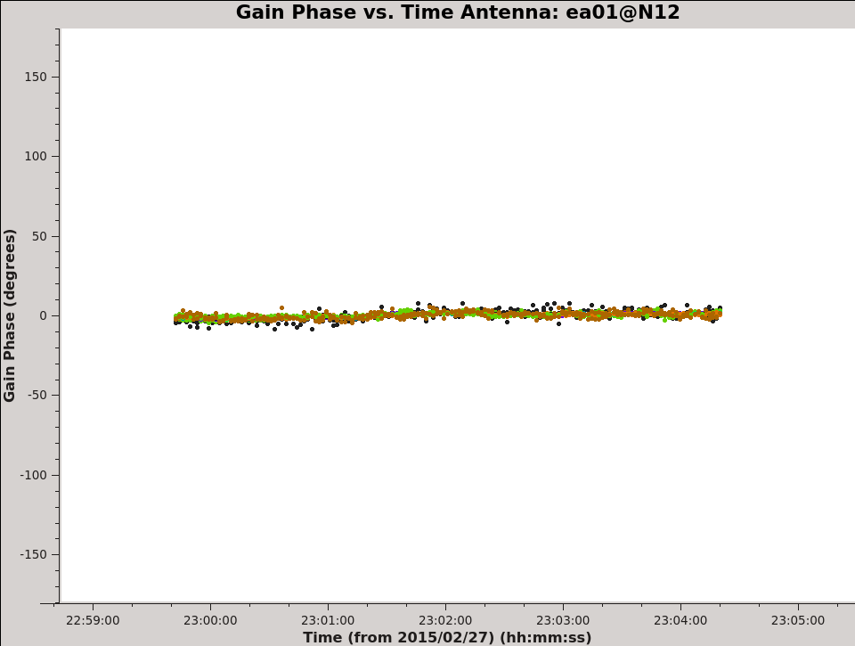
Similar to the bandpass flagging, we will flag outlier gain solutions in both amplitude and phase. For the amplitudes, the final scatter around an average close to one should be a few percent (see Fig. 8a,b). Note antennas ea08, ea09 have particularly noisy solutions. Remember that the gain solutions for both polarizations can be flagged together, as we will lose the equivalent data of the surviving polarization anyway.
Note that when plotting gains against time, it is convenient to use auto-scaling of the time axis by putting 0 in the first two fields of plotrange.
 |
 |
Next, we will prepare a smoothed and interpolated version of the gain calibration table using task smoothcal, which will be applied later to the target field data. This prevents flagging of target field data when one of the edges of a calibrator scan is flagged for one or more antennas. The CalTable results from smoothing can be inspected with plotms.
# In CASA
smoothcal(vis='3C129_pband.ms', tablein='3C129_pband.G1', caltable='3C129_pband.Gs1', smoothtype='median', smoothtime=60.*60.)
#
plotms(vis='3C129_pband.Gs1', xaxis='time', yaxis='amp', iteraxis='antenna', plotrange=[0,0,0.8,1.2], coloraxis='spw')
#
plotms(vis='3C129_pband.Gs1', xaxis='time', yaxis='phase', iteraxis='antenna', plotrange=[0,0,-10.,10.], coloraxis='spw')
Transfer of calibrations to the target field
So far we have used one scan on the primary calibrator 3C147 to derive various calibration tables. These calibrations will now be applied to all scans of all sources in our measurement set, which includes 3C147 itself and our target field 3C129. As described above, the task applycal creates a CORRECTED_DATA column in which the calibrated visibilities get stored. This may take a while.
# In CASA
applycal(vis='3C129_pband.ms', parang=True, applymode='calflagstrict', flagbackup=True, gaintable=['3C129_pband.antpos','3C129_pband.rq',
              '3C129_pband.tecim','3C129_pband.K1','3C129_pband.B1','3C129_pband.Gs1'],
         interp=['','','','nearest,nearestflag','nearest,nearestflag','nearest,nearestflag'])
Now we split off the calibrated target field data, meaning that the visibilities of source 3C129 get copied from the CORRECTED_DATA column to the DATA column of a new measurement set. This is convenient for further processing.
# In CASA
split(vis='3C129_pband.ms', outputvis='3C129_pband_target.ms', datacolumn='corrected', field='3C129')
It is also helpful to perform additional flagging for any residual RFI left behind in our target after all our calibration steps have been completed before we begin the imaging of our data.
flagdata(vis='3C129_pband_target.ms', mode='rflag')
flagdata(vis='3C129_pband_target.ms', mode='extend')
Statwt
Before we go ahead and image our target field we should try to downweight any low level residual RFI. This is done using the task statwt. The task computes the rms of the data, weighting down outliers. This makes a big impact for imaging of a target in the presence of low level residual RFI. For our purposes we will bin the data in a time interval larger than the integration time as follows.
# In CASA
statwt(vis='3C129_pband_target.ms', datacolumn='data', timebin=30)
With data weights for outliers being set we will now proceed with the imaging and self-calibration of our data.
Imaging
At this point, we're ready to make a first image of our target field. Imaging in CASA is done by means of the tclean task. The task implements algorithms for wide field imaging, such as W-Projection (Cornwell et al. 2008 http://arxiv.org/abs/0807.4161) and Multi Term Multi Frequency Synthesis (Rau et al. 2011 http://arxiv.org/abs/1106.2745) both of which we will utilize to make our initial image, even though the radio galaxy lies in the center of our field. The observations were carried out in B configuration resulting in an effective maximum resolution of approximately 5x5 arcsecs. To effectively model the source spectral index in the sky, we will utilize the mtmfs algorithm and the wproject algorithm to make a wide field image (the full beam at P Band is about 3 degrees in diameter). So, going by these requirements, we can now compute the required cell and image sizes. Consulting the NRAO science page on resolution, we can see that the expected HPBW for B Configuration, P Band is 18.5 arcsec. So, we can sample it well by using a 5 arcsec cellsize. Having done that, if we decide to make a wide field image to account for all the point sources we will set the image size parameter to 4860 pixels. To enable the wide-field algorithm, we set gridder='wproject': this invokes the W-Projection algorithm, upon which we set the number of W-Projection planes to be 128. We set the deconvolution mode as Multi Term Multi Scale Multi Frequency Synthesis using the deconvolver='mtmfs' parameter. We set the number of Taylor terms to be considered during imaging to be 2. This allows for the source spectral variation to be modeled by a second degree (first order) polynomial. We choose three different scales to model the point source and extended emission in our field well by setting scales=[0,20,30]. We launch the interactive tclean process, but only for spw='3~8' to begin with. Note, running the first clean call will take at least ~10 min to process.
# In CASA
tclean(vis='3C129_pband_target.ms', imagename='3C129_initial_clean', cell=['5.0arcsec','5.0arcsec'], imsize=[4860,4860], deconvolver='mtmfs',
         nterms=2, gridder='wproject', wprojplanes=128, stokes='I', niter=20000, spw='3~8', interactive=True, scales=[0,20,30],
         pblimit=0.01, savemodel='modelcolumn', weighting='briggs', robust=0.0)
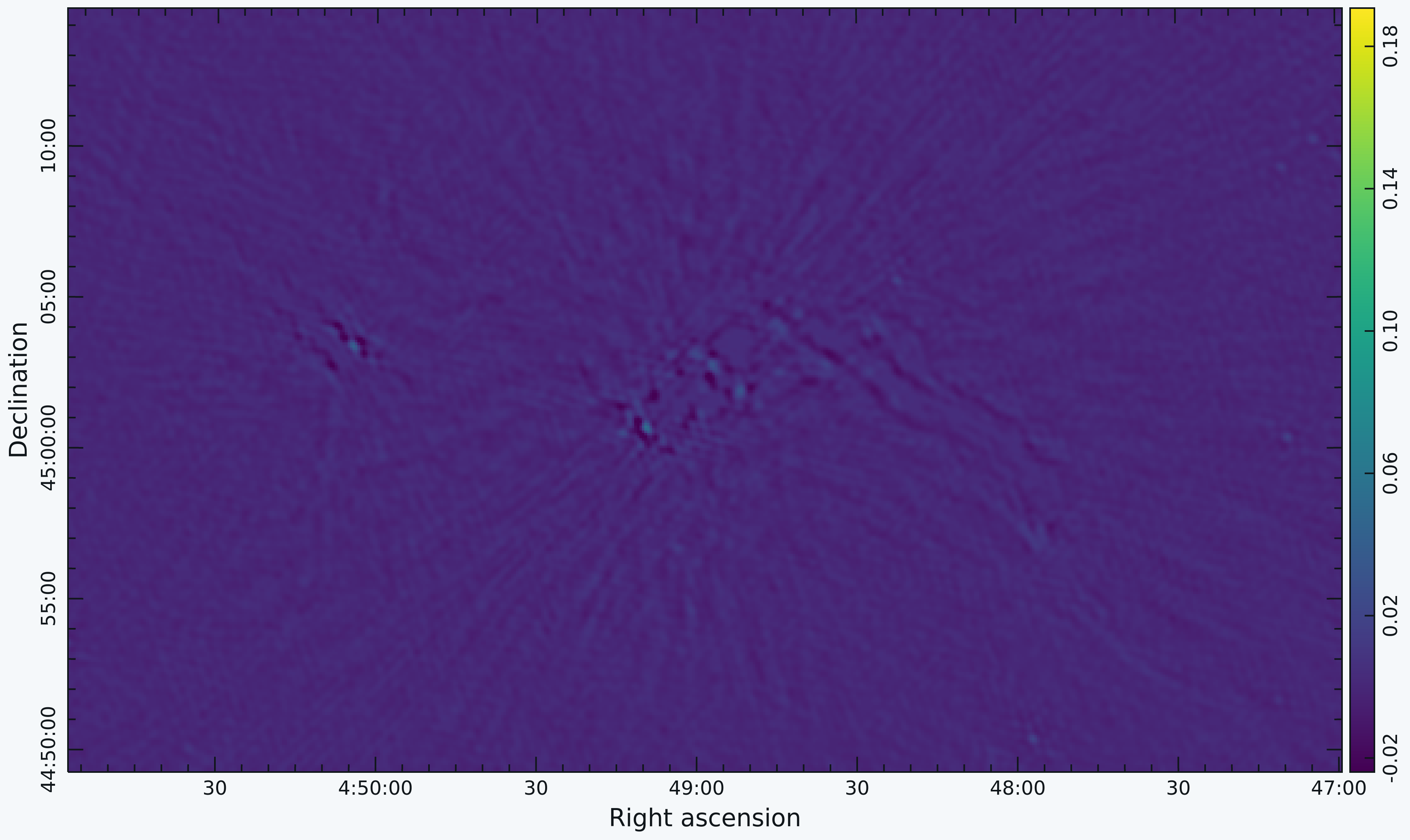
The tclean command launches an interactive session after 100 iterations of cleaning and produces a wide field map with two sources at the center and a lot of bright sources far out in the field (Fig. 9a). As it is a snapshot image, the bright sources have significant side lobes and so tight clean boxing can help. This can be done in the interactive viewer interface that pops up. If we proceed with interactive tclean with subsequent steps to keep boxing out the strong sources that pop up in the image, we finally see the extended emission from the target radio galaxy begin to emerge. Continue boxing and cleaning to ensure that the residuals of the boxed cleaning look noise like (~10000 iterations). We now stop the interactive task and look at the final image it produced (Fig. 9b).
# In another terminal outside CASA
carta 3C129_initial_clean.image.tt0
 |
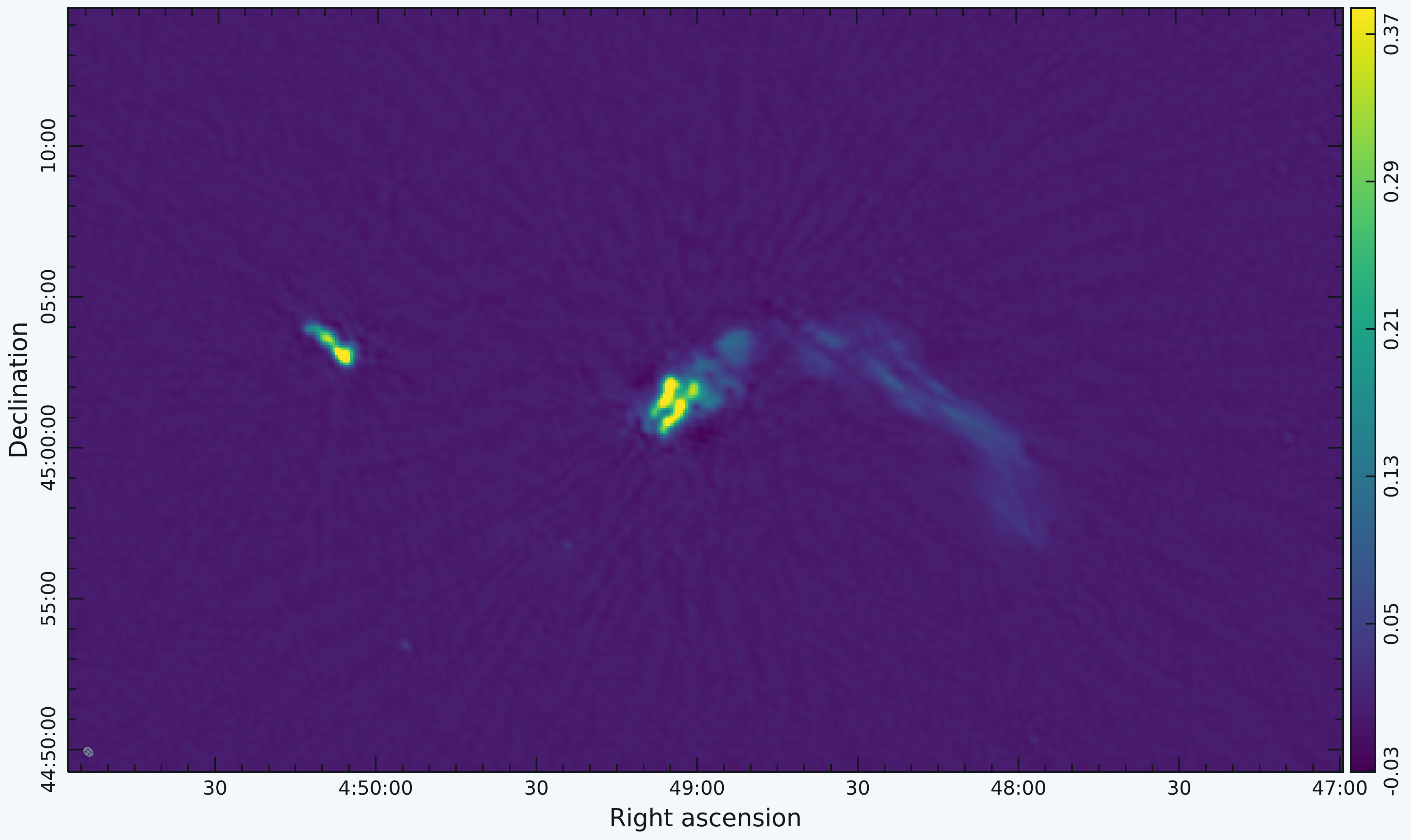 |
The recovered structure at the center of the map should resemble what is shown in Fig. 9b. If the image looks worse, then boxing of bright features in the map needs to be done more carefully. Note the image has some sources still showing strong side lobes and imaging artifacts around them. We expected this as we have carried out phase calibration only on our flux calibrator and have just transferred the solutions over to our target field. Since we used savemodel='modelcolumn', the MODEL_DATA column in the measurement set now contains the initial image model, which we will self calibrate against to produce a better image. Also notice that the spw's utilized are the cleanest spectral windows that are totally RFI free.
Self Calibration
We now proceed to compute gain phase solutions for our target field using the tasks gaincal, bandpass, and applycal as the first step in self-calibration. For a full guide on self-calibration process, please see the Self-calibration CASA tutorial.
# In CASA
gaincal(vis='3C129_pband_target.ms', caltable='3C129_pband_target.ScG0', field='3C129', solint='inf', refant='ea09',
           spw='3~8', minsnr=3.0, gaintype='G', parang=True, calmode='p')

bandpass(vis='3C129_pband_target.ms', caltable='3C129_pband_target.ScB0', field='3C129', solint='inf', refant='ea09', minsnr=3.0, spw='3~8',
                parang = True, gaintable=['3C129_pband_target.ScG0'], interp=['','','','nearest,nearestflag'])

applycal(vis='3C129_pband_target.ms', gaintable=['3C129_pband_target.ScG0','3C129_pband_target.ScB0'], spw='3~8', applymode='calflagstrict')
Having applied these gain and bandpass solutions, we will once again image the target measurement set which we now expect to have better gain solutions and consequently a better image. We do this by invoking the tclean command once again.
# In CASA
tclean(vis='3C129_pband_target.ms', imagename='3C129_clean_sc0', cell=['5.0arcsec','5.0arcsec'], imsize=[4860,4860], deconvolver='mtmfs',
         nterms=2, gridder='wproject', wprojplanes=128, stokes='I', niter=20000, spw='3~8', interactive=True, scales=[0,20,30],
         pblimit=0.01, savemodel='modelcolumn', weighting='briggs', robust=0.0)

# In terminal
carta 3C129_clean_sc0.image.tt0
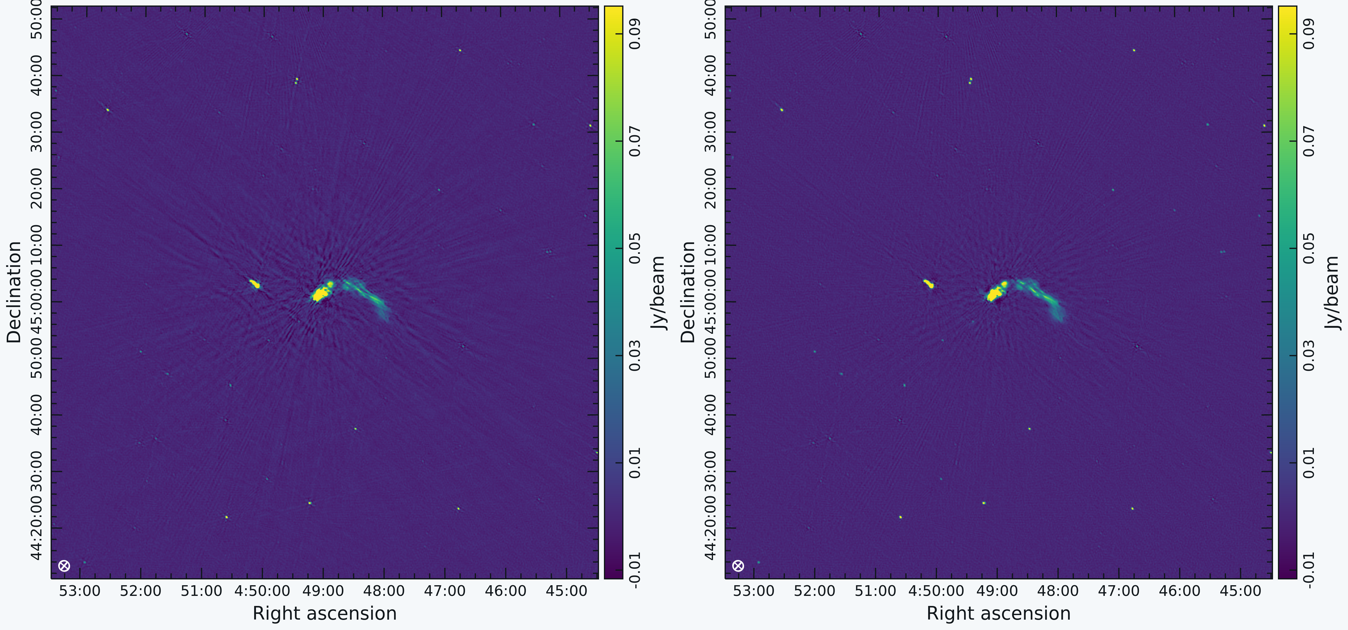
On boxing and cleaning, we already notice that the imaging artifacts have reduced significantly. We also see that the target source appears to contain more structure and a greater amount of flux. Further self calibration iterations involving an amplitude & phase gain calibration, and target bandpass calibration, are all possible steps that can be explored. Example on the final improvements the self-calibration can provide is shown in Fig. 10.
 |
Appendix: Some P-band data issues you may want to know about
Unfortunately, there are a few known issues with the upgraded VLA P-band observing. Most problems were discovered during the P-band commissioning period and have been fixed for newer data sets, but the archive keeps part of this history alive. Here we will go over some of those issues, and (if possible) provide ways of fixing them.
Double data descriptor entries
The data description table is part of the measurement set, and provides a link between the recorded visibilities, the spectral window information and the polarization information. For some data sets, the data description table contains two entries for each P-band spectral window, one pointing towards a circular (RL) polarization definition, and one pointing towards a linear (XY) polarization definition. A contributed task fixlowband() is available to recognize and fix this problem.
Continuous Radio Frequency Interference (RFI)
The wide bandwidth of the low-band receiver is (unfortunately) guaranteed to contain significant amounts of RFI. There are a few RFI sources that are active all the time, and are visible in all array configurations. The default P-band observing setup of 16 x 16 MHz tries to capture as much of the continuous RFI in as few spectral windows as possible, allowing for a simple RFI mitigation strategy in which these spectral windows (spws 1,2 and 9,10, but possibly more) can be immediately flagged.
Two spectral window setup
In the early commissioning period of the VLA upgrade, the default setup for P-band observing was to use 2 spectral windows of 1024 channels each to cover 256 MHz of bandwidth from 230 MHz to 486 MHz. However, it was noticed that strong, narrow-band RFI events were causing data to be lost for the whole spectral window in which they occurred. To make the system more robust against data loss from such events, the frequency range was divided into 16 x 16 MHz, and shifted downwards by 6 MHz to capture ever-present RFI into as few spectral windows as possible. If your data has only two P-band spectral windows, please be aware that a higher data loss due to RFI is possible. There is no way to repair this.
Bandpass ripples
Due to signal reflections in cables and within the VLA dish, sinusoidal amplitude and phase modulations are always present in P-band data. This is most easily seen in bandpass calibration plots of amplitude versus frequency. In some cases, mostly due to cable & connector problems, these modulations can be very strong (~up to 50 percent of the average amplitude level). These modulations tend not to vary over the duration of an observation and can therefore be removed through bandpass and polarization calibration. If they are found to be variable (e.g., by inspecting bandpass solutions for separate calibrator scans), the offending antenna / polarization should be flagged.
High cross-polarization
On each antenna, the P-band feed (dipole) is visually aligned with respect to the primary focus support legs. This is normally done within 5-10 degrees accuracy. On rare occasions the dipole on one antenna has accidentally rotated to much larger angles because the locking bolt on the back of the feed was not completely tightened. The result is a high cross-polarization in the baseline visibilities that include this antenna. If this is the case, it is safest to flag this data, since there is a possibility that the dipole has rotated during the observations.
Instrumental Polarization Calibration
While polarization leakage calibration has been highlighted in the past reports, it does not directly impact imaging in Stokes I and hence has been dropped from this casaguide.
Useful links
- The EVLA Low-Band Receiver System Status & User Pages
- VLA Very Low Frequency Observing
- Here is a link to a script that will run this CASA guide automatically: VLARadiogalaxy3C129P-bandcontinuumtutorial-CASA6.5.4
Last checked on CASA Version 6.5.4