Simulation Guide Component Lists (CASA 4.4)
This guide is applicable to CASA version 4.4.
To create a script of the Python code on this page see Extracting scripts from these tutorials.
Explanation of the guide
When writing an interferometric proposal it is often useful to simulate observations of very simple objects, like point sources, Gaussians, and disks. In CASA, observations can be simulated using task simobserve and analyzed using task simanalyze. This guide demonstrates how to simulate ALMA observations of a Gaussian and some point sources using these tasks and using the CASA Toolkit.
We begin by employing component lists in the Toolkit to create an image of a Gaussian flux distribution, which will be saved as a FITS file. The fits file will then be "observed" using simobserve and simanalyze along with four point sources, added via the componentlist parameter. Finally, we show how the same observations could have been done without any skymodel in simobserve, instead using only component lists.
Getting Started
To get started you need CASA version 4.4.
To install CASA, follow the instructions given on the Obtaining CASA page.
CASA Basics
CASA is the post-processing package for ALMA and EVLA and can handle both interferometric and single dish data. To get a brief introduction to simobserve and simanalyze, the tasks within CASA that we will use here, go to the Simulation Guide for New Users. To learn more about CASA in general, go to the CASA homepage. Walk-throughs of CASA data reduction for a variety of data sets can be found on the CASA Guides website.
Once you have installed CASA, you can launch it by typing "casapy" at the prompt or by double-clicking on the icon, depending on your system and preferences.
Making a Simple FITS Image
Here we show how to create a simple FITS image using the CASA tasks and the toolkit. The example here will be that of a Gaussian flux distribution. Enter the following lines at the CASA prompt:
# In CASA
direction = "J2000 10h00m00.0s -30d00m00.0s"
cl.done()
cl.addcomponent(dir=direction, flux=1.0, fluxunit='Jy', freq='230.0GHz', shape="Gaussian",
                majoraxis="0.1arcmin", minoraxis='0.05arcmin', positionangle='45.0deg')
#
ia.fromshape("Gaussian.im",[256,256,1,1],overwrite=True)
cs=ia.coordsys()
cs.setunits(['rad','rad','','Hz'])
cell_rad=qa.convert(qa.quantity("0.1arcsec"),"rad")['value']
cs.setincrement([-cell_rad,cell_rad],'direction')
cs.setreferencevalue([qa.convert("10h",'rad')['value'],qa.convert("-30deg",'rad')['value']],type="direction")
cs.setreferencevalue("230GHz",'spectral')
cs.setincrement('1GHz','spectral')
ia.setcoordsys(cs.torecord())
ia.setbrightnessunit("Jy/pixel")
ia.modify(cl.torecord(),subtract=False)
exportfits(imagename='Gaussian.im',fitsimage='Gaussian.fits',overwrite=True)

The first line defines a string "direction" which will be the center of the Gaussian flux distribution.
cl.done closes any open component lists, if any.
cl.addcomponent creates a new component centered at "direction", with a flux of 1 Jy at a frequency of 230 GHz, a Gaussian shape of 0.1 by 0.05 arcminutes, and a position angle of 45 degrees.
ia.fromshape creates a new, empty CASA image with the name and dimensions given.
cs=ia.coordsys gets the coordinate system of the image.
cs.setunits defines the units of the four axes of the new CASA image.
cell_rad will be the cell size and units in this CASA image, 0.1 arcseconds.
cs.setincrement tells CASA that RA increases to the right, Dec increases going up, and, a few lines later, that the one channel is 1 GHz wide.
cs.setreferencevalue sets the center of the image in RA, Dec, and frequency.
ia.setcoordsys puts the coordinates and frequencies into the image header.
ia.setbrightnessunit defines the brightness unit (Jy per pixel) of the CASA image.
ia.modify puts the Gaussian component into the image.
exportfits writes the resultant CASA image as a FITS file (not strictly necessary since you can run simobserve on Gaussian.im, but useful to know in general).
As usual, more information can be found via the help in CASA:
# In CASA
help(ia.modify)  # syntax for help with toolkit or CASA tasks
help("exportfits") # syntax for help with CASA tasks, but not the toolkit
Simulating Observations with a FITS Image and a Component List
One use for component lists would be to simulate the effect of having one or more point sources added to an input image, with the goal of finding out the effect on the simulated observations. For instance, one might want to know if a faint point source would be detectable if there is extended emission around it. Conversely, one might want to know if the artifacts from imaging a field with a bright point source would make a project tricky to carry out. In this example, we will use component lists in the simobserve task to add four point sources to an input FITS image. The input image will be the Gaussian flux distribution created above.
First we create the four point sources using the CASA toolkit:
# In CASA
os.system('rm -rf point.cl')
cl.done()
cl.addcomponent(dir="J2000 10h00m00.08s -30d00m02.0s", flux=0.1, fluxunit='Jy', freq='230.0GHz', shape="point")
cl.addcomponent(dir="J2000 09h59m59.92s -29d59m58.0s", flux=0.1, fluxunit='Jy', freq='230.0GHz', shape="point")
cl.addcomponent(dir="J2000 10h00m00.40s -29d59m55.0s", flux=0.1, fluxunit='Jy', freq='230.0GHz', shape="point")
cl.addcomponent(dir="J2000 09h59m59.60s -30d00m05.0s", flux=0.1, fluxunit='Jy', freq='230.0GHz', shape="point")
cl.rename('point.cl')
cl.done()
First we delete any previous version of the file 'point.cl', which will be the output file created in a few lines. Then we use cl.done to begin and end this sequence to close any open component list. The cl.addcomponent commands create point sources that are 0.1 Jy at 230 GHz at the coordinates given in each line. The cl.rename command tells CASA the name of output component list file.
We use simobserve and simanalyze to make the simulated observations of these point sources and the Gaussian flux distribution given in the FITS file we made previously in this guide.
# In CASA
default("simobserve")
project = "FITS_list"
skymodel = "Gaussian.fits"
inwidth = "1GHz"
complist = 'point.cl'
compwidth = '1GHz'
direction = "J2000 10h00m00.0s -30d00m00.0s"
obsmode = "int"
antennalist = 'alma.cycle0.compact.cfg'
totaltime = "28800s"
mapsize = "10arcsec"
thermalnoise = ''
simobserve()
#
default("simanalyze")
project = "FITS_list"
vis="FITS_list.alma.cycle0.compact.ms"
imsize = [256,256]
imdirection = "J2000 10h00m00.0s -30d00m00.0s"
cell = '0.1arcsec'
niter = 5000
threshold = '10.0mJy/beam'
analyze = True
simanalyze()
To learn more about simobserve and simanalyze, look at the Simulation Guide for New Users. Here we simulate observations of the Gaussian flux distribution (given with the skymodel parameter) with the point sources (given with the complist parameter) using simobserve. We center the observations at the center of the Gaussian flux distribution and the point sources, and the field to be imaged is 20" by 20". We simulate 8 hours (28800 seconds) of observations with ALMA in the Cycle 0 compact array configuration. The simobserve task puts the u-v data in a measurement set called "FITS_list.alma.cycle0.compact.ms" (inside the "FITS_list" project directory), and this will be the input to make a map of the emission.
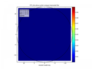
Figure 2: The skymodel.png graphic produced by simobserve has non-optimal scaling (under development)
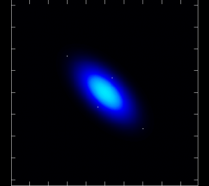
Figure 3: Loading the skymodel.flat image in the viewer reveals the broad Gaussian in addition to the compact components.


A subtlety of simulating with components and an image skymodel is that the skymodel image created in the simulation directory is only the (scaled) input image, while skymodel.flat contains that image plus the list of components inserted into it.
Inverting the u-v data and making a clean (deconvolved) map of the flux distribution is done with the simanalyze task in CASA. The purpose of this guide is to illustrate the use of component lists, not to make the best possible image of this simple flux distribution, so we don't take much care to do the best possible job with the cleaning. For instance, we don't use a mask or clean boxes, nor do we clean interactively to make sure that there is no point in cleaning further. To see a thorough explanation of imaging and deconvolution, see the CASA guides for ALMA science verification data, for instance Antennae Band 7 or TW Hydra Band 7
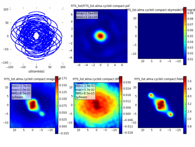
Figure 4: simulated observations of a Gaussian (skymodel) and four point sources (component list) - analysis.png image created by simanalyze.

Simulating Observations with Just a Component List
The CASA task simobserve can be run on a simulated sky given entirely by the complist parameter, with nothing given in the skymodel parameter. A simulation of observations of a Gaussian plus four point sources can be accomplished with only component lists, as shown in the example below.
# In CASA
os.system('rm -rf Gauss_point.cl')
cl.done()
cl.addcomponent(dir="J2000 10h00m00.00s -30d00m00.0s", flux=1.0, fluxunit='Jy', freq='230.0GHz', shape="Gaussian",
                majoraxis="0.1arcmin", minoraxis='0.05arcmin', positionangle='45.0deg')
#
cl.addcomponent(dir="J2000 10h00m00.08s -30d00m02.0s", flux=0.1, fluxunit='Jy', freq='230.0GHz', shape="point")
cl.addcomponent(dir="J2000 09h59m59.92s -29d59m58.0s", flux=0.1, fluxunit='Jy', freq='230.0GHz', shape="point")
cl.addcomponent(dir="J2000 10h00m00.40s -29d59m55.0s", flux=0.1, fluxunit='Jy', freq='230.0GHz', shape="point")
cl.addcomponent(dir="J2000 09h59m59.60s -30d00m05.0s", flux=0.1, fluxunit='Jy', freq='230.0GHz', shape="point")
cl.rename('Gauss_point.cl')
cl.done()
Here we have created a Gaussian flux distribution with the same properties as in the FITS image created above. Surrounding the Gaussian are four point sources with the same positions and brightness as before. The only difference between this call to simobserve and the one above is that here the Gaussian flux distribution is included in the component list instead of being defined by a FITS file.
# In CASA
default("simobserve")
project = "complist_only"
complist = 'Gauss_point.cl'
compwidth = '1GHz'
direction = "J2000 10h00m00.0s -30d00m00.0s"
obsmode = "int"
antennalist = 'alma.cycle0.compact.cfg'
totaltime = "28800s"
mapsize = "10arcsec"
thermalnoise = ''
simobserve()
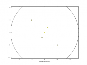
Figure 5: Note that in the case of component-only simulation, the skymodel graphic produced simply shows the component positions as points.

The simulated visibilities and images are essentially identical, as seen in the analysis.png produced by simanalyze.
default("simanalyze")
project = "complist_only"
vis="complist_only.alma.cycle0.compact.ms"
imsize = [256,256]
imdirection = "J2000 10h00m00.0s -30d00m00.0s"
cell = '0.1arcsec'
niter = 5000
threshold = '10.0mJy/beam'
analyze = True
simanalyze()
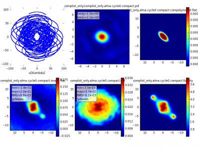
Figure 6: Simulated observations of a Gaussian and four point sources, all input using the component list.

However, there are some subtle differences. When simulating from a componentlist only, simobserve creates a skymodel image for display purposes (the visibilities are calculated directly from the componentlist). The choice of pixel size in that display image (called "compskymodel" and "compskymodel.flat") is based on an estimate of the eventual clean beam size, and may not be the same pixel size as defined by for a user-input skymodel image (e.g., the 0.1" pixel chosen for Gaussian.im earlier in this guide). As the skymodel and compskymodel images are displayed with units of Jy/pixel, different pixel sizes result in different numerical values, even for the same total flux. Furthermore, any unresolved components are placed in a single pixel of the compskymodel image (or in the case of image plus componentlist input, into the skymodel.flat image). If the pixel sizes differ significantly, then the position of the source can also differ by as much as a pixel.
The most important aspects of the simulation are the visibilities and the corresponding simulated (observed) sky image; these are the same for the componentlist+skymodel and the componentlist-only (compare the bottom left plot in Figure 4 and Figure 6 on this page). However, the small differences in the generated input images (resulting from different pixel sizes) can result in large changes in the difference image. This is the same case as when, e.g., subtracting a continuum image from a narrow-band CCD image of stars - misalignment by as little as 0.1 pixel can produce visually dramatic residuals in the continuum-subtracted image.
Thus, when the difference and fidelity images for these two methods are compared, one will find small differences due to these pixelization effects. In general, for simulations you are advised to use pixels significantly smaller than the clean beam (simobserve prints warnings when this is not the case), and to be careful of interpreting features of simulated images at dynamic range greater than about 100.