Einstein-Face (CASA 4.4)
This guide is applicable to CASA version 4.4. For simulation instructions for older versions of CASA see: Einstein-Face (CASA 4.3).
Simulations using non-science images: the face of Einstein
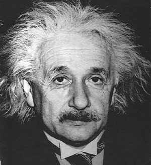
simobserve can be used to simulate an observation of any digitized image, and simanalyze can be used to image and analyze the data from that simulated observation. These toy models can be particularly useful for examining the effects of varying uv-coverage on image fidelity. In this example we use a photo of Albert Einstein as the input model.
We start with a JPG image of Einstein's face. simobserve likes input images in FITS format, so we used Gimp to convert the file. (Instructions to Convert jpg to fits.) The original image is shown below. You can grab the converted FITS file directly here or from the Simulation Inputs CASA Guide page.
Prepare inputs for simobserve
We will start with a 10 minute observation using one of the "full science" antenna configurations. Inputs to simobserve and simanalyze are given below. The integration time (300 s) is set much longer than we would see in a real ALMA observation (1 to 10 s) to speed the computation. We set the angular size of the image to 0.043 arcsecond pixels with the incell parameter, ensuring that only one pointing is needed to map the whole image area. The image coordinates are set to a position near the Chandra Deep Field South.
# simobserve is used to simulate the observation
default('simobserve')
# Full science, configuration 08, 10 minutes
project = 'fs_cfg8_10m'
skymodel = 'Einstein.fits'
indirection = 'J2000 03h30m00 -28d00m00'
incell = '0.043arcsec'
incenter = '245GHz'
inwidth = '2GHz'
setpointings = T
integration = '300s'
mapsize = ['1arcmin','1arcmin']
maptype = 'hexagonal'
pointingspacing = '1arcmin'
graphics = 'both'
obsmode = 'int'
antennalist =  "alma.out08.cfg"
totaltime = '600s'
thermalnoise = ""
simobserve()
An aside about antenna configurations
ALMA will observe with many different array configurations. In our simulations we can specify which antenna configuration to use with the antennalist parameter. Your CASA distribution comes with a set of antenna configurations. A list of configuration files available in CASA 4.1 is available here. Also, you can locate the configurations like so:
CASA <49>: print os.getenv('CASAPATH').split(' ')[0] + '/data/alma/simmos/'
/usr/lib64/casapy/stable/data/alma/simmos/
CASA <50>: ls /usr/lib64/casapy/stable/data/alma/simmos/
aca_cycle1.cfg            alma.out05.cfg  alma.out21.cfg  pdbi-c.cfg
aca.i.cfg                 alma.out06.cfg  alma.out22.cfg  pdbi-d.cfg
aca.ns.cfg                alma.out07.cfg  alma.out23.cfg  sma.compact.cfg
aca.tp.cfg                alma.out08.cfg  alma.out24.cfg  sma.compact.n.cfg
alma.cycle0.compact.cfg   alma.out09.cfg  alma.out25.cfg  sma.extended.cfg
alma.cycle0.extended.cfg  alma.out10.cfg  alma.out26.cfg  sma.subcompact.cfg
alma_cycle1_1.cfg         alma.out11.cfg  alma.out27.cfg  sma.vextended.cfg
alma_cycle1_2.cfg         alma.out12.cfg  alma.out28.cfg  vla.a.cfg
alma_cycle1_3.cfg         alma.out13.cfg  carma.a.cfg     vla.b.cfg
alma_cycle1_4.cfg         alma.out14.cfg  carma.b.cfg     vla.bna.cfg
alma_cycle1_5.cfg         alma.out15.cfg  carma.c.cfg     vla.c.cfg
alma_cycle1_6.cfg         alma.out16.cfg  carma.d.cfg     vla.cnb.cfg
alma.out01.cfg            alma.out17.cfg  carma.e.cfg     vla.d.cfg
alma.out02.cfg            alma.out18.cfg  meerkat.cfg     vla.dnc.cfg
alma.out03.cfg            alma.out19.cfg  pdbi-a.cfg      WSRT.cfg
alma.out04.cfg            alma.out20.cfg  pdbi-b.cfg
Imaging with simanalyze
Now back to the simulation. Execute simanalyze with the following parameters:
# simanalyze is used to take the simulation output, and provide helpful plots
default('simanalyze')
project = 'fs_cfg8_10m'
image = T
vis = project+'.alma.out08.ms'
imsize = [300,300]
cell = '0.043arcsec'
niter = 2000
weighting = 'natural'
analyze = F
overwrite = T
simanalyze()
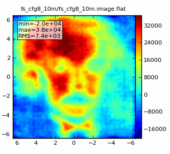
The output image should have a clean beam of 0.62"x0.56" and look something like:
Experimenting with longer observations and different array configurations
We can repeat the simulation, this time for an 1 hr observation:
tget(simobserve)
# Full science, configuration 08, 1 hour
project = 'fs_cfg8_1hr'
totaltime = '3600s'
simobserve()
tget(simanalyze)
project = 'fs_cfg8_1hr'
vis = project+'.alma.out08.ms'
simanalyze()
The result should look something like: 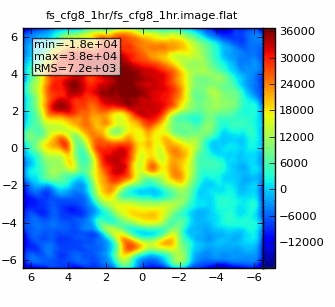
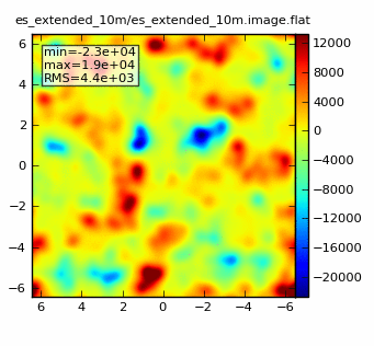
Next, we can see the result of observing this model image with the Early Science extended antenna configuration. First we use a 10 min observation:
tget(simobserve)
project = 'es_extended_10m'
antennalist = "alma.cycle0.extended.cfg"
totaltime = '600s'
simobserve()
tget(simanalyze)
project = 'es_extended_10m'
vis = project+'.alma.cycle0.extended.ms'
simanalyze()
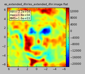
We see the limited ability of the Early Science configuration for imaging complex structure with short observations. Next we can try a 4 hr observation, using the same configuration.
tget(simobserve)
project = 'es_extended_4hr'
totaltime = '14400s'
simobserve()
tget(simanalyze)
project = 'es_extended_4hr'
vis = project+'.alma.cycle0.extended.ms'
simanalyze()
Going back to one of the Full Science, compact array configurations, we can simulate an 8 hr observation to show the improvement obtained by obtained by filling in uv-coverage.
tget(simobserve)
antennalist = "alma.out08.cfg"
project = 'fs_cfg8_8hr'
totaltime = '28800s'
simobserve()
tget(simanalyze)
project = 'fs_cfg8_8hr'
vis = project+'.alma.out08.ms'
simanalyze()
Which should look something like: 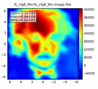
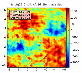
We can simulate an observation using a Full Science, extended configuration to achieve high spatial resolution. In this case there are no short spacings and we will see the drastic effects of missing those. We select configuration 16, which has a 0.17x0.15 beam, still better than Nyquist sampling of the model image (which has 0.043" pixels).
tget(simobserve)
antennalist = "alma.out16.cfg"
project = 'fs_cfg16_1hr'
totaltime = '3600s'
simobserve()
tget(simanalyze)
project = 'fs_cfg16_1hr'
vis = project+'.alma.out16.ms'
simanalyze()
The lack of short spacings in the configuration leads to poorly sampled structure on large spatial scales. In practice, one would need to combine observations using this configuration with a set in a more compact configuration (such as 8) to sample both the large and small spatial structures.
