EVLA high frequency Spectral Line tutorial - IRC+10216 part2-CASA3.3
This is the second part of the EVLA IRC+10216 data reduction tutorial. IRC+10216-CASA3.3 Part 1: editing, calibration
UV Continuum Subtraction and Setting Up for Self-Calibration
Now we can make a vector averaged uv-plot of the calibrated target spectral line data. It is important to note that you will only see signal in such a plot if (1) the data are well calibrated, and (2) there is significant signal near the phase center of the observations, or if the line emission (or absorption) is weak but extended. If this isn't true for your data, you won't be able to see the line signal in such a plot and will need to make an initial (dirty or lightly cleaned) line+continuum cube to determine the line-free channels. Generally, this is the recommended course for finding the line-free channels more precisely than is being done here due to time constraints, as weak line signal would not be obvious in this plot.
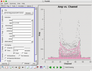
plotms(vis='IRC10216',field='',ydatacolumn='corrected',
       xaxis='channel',yaxis='amp',correlation='RR',
       avgtime='1e8',avgscan=T,spw='0~1:4~60',antenna='', coloraxis='spw')
In the Display tab, change the Unflagged Points Symbol to Custom and Style of 3.
You should see the "horned profile" typical of a rotation shell. From this plot, you can guess that strong line emission is restricted to channels 18 to 47 (zoom in if necessary to see exactly what the channel numbers are).
In the Data tab, under Averaging, you can also click on "All Baselines" to average all baselines, but this is a little harder to see.
Now we want to use the line free channels to create a model of the continuum emission that can be subtracted to form a line-only dataset. We want to refrain from going to close to the edges of the band -- these channels are typically noisy, and we don't want to get too close to the line channels because we could only see strong line emission in the vector averaged uv-plot.
uvcontsub2(vis='IRC10216',fitspw='0~1:4~13;52~60',
       want_cont=T)
The "want_cont=T" will produce two new datasets, IRC10216.contsub is the continuum subtracted line data, and IRC10216.cont is the continuum estimate (note however, that it is still a multi-channel dataset).
Velocity Systems and Doppler corrections
The current incarnation of the EVLA does not support Doppler tracking. Doppler setting is possible which will calculate the sky frequency based on a velocity of the source at the start of an observation. The sky frequency is then fixed throughout that track. Typically, a fixed frequency is better for the calibration of interferometric data. The downside, however, is that ta spectral line may shift over one or more channels during an observation. clean takes care of such a shift when regridding the visibilities in velocity space (default is LSRK) to form an image. Sometimes, in particular when adding together different observing tracks, it may be advisable to do the regrid all data sets to the same velocity grid, combine all data to a single file, then Fourier transform and deconvolve. The tasks cvel, concat, and clean serve this purpose respectively. The following run of cvel shows an example on how the parameters of cvel may be set.
The IRC10216.contsub visibility spans the following channel range (see also the listobs output in the first part of the tutorial):
# In CASA
vishead(vis='IRC10216.contsub', mode='summary')
SpwID  #Chans Frame Ch1(MHz)    ChanWid(kHz)  TotBW(kHz)  Corrs
0          64 TOPO  36387.2295  125           8000        RR  RL  LR  LL
1          64 TOPO  36304.542   125           8000        RR  RL  LR  LL
For spw 0, this corresponds to about 1 km/s channel width. If we want to image the HC3N spectral line with a rest frequency of 36.39232 GHz over a velocity range of -50km/s to 0km/s and a channel width of 5 km/s, we may decide to regrid the visibilities in cvel as
Note that this step is not necessary for the processing further down in this tutorial. You may skip it if you wish.
# In CASA
cvel(vis='IRC10216.contsub', outputvis='IRC10216.contsub-cveled', mode='velocity',
     interpolation='linear', nchan=10, start='-50km/s', width='5km/s',
     restfreq='36.39232GHz',outframe='LSRK', veltype='optical')
This will create a new dataset where the data is binned into the new grid. Since all data in measurement sets are stored in frequency space, an inspection with vishead now gives:
# In CASA
vishead(vis='IRC10216.contsub-cveled', mode='summary')
SpwID  #Chans Frame Ch1(MHz)    ChanWid(kHz)  TotBW(kHz)  Corrs
0          10 LSRK  36392.927   606.97375     6070.64874  RR  RL  LR  LL
After the cvel step, the data can then be combined with other observations via concat and imaged in clean with mode='channel' to conserve that velocity system and grid.
Note that cvel can also Hanning smooth the data, if needed (as an alternative to the stand-alone hanningsmooth task).
Image the Spectral Line Data
Here we make images from the continuum-subtracted, calibrated spectral line data. Because the spectral line emission from IRC+10216 has significant extended emission, it is very important to run clean interactively, and make a clean mask. To make the cube a bit smaller and stay away from noisy edge channels we restrict the channel range using the spw parameter.
Note that interrupting clean by Ctrl+C may corrupt your visibilities -- you may be better off choosing to let clean finish. We are currently implementing a command that will nicely exit to prevent this from happening, but for the moment try to avoid Ctrl+C.
# In CASA
clean(vis='IRC10216.contsub',imagename='IRC10216_HC3N.cube_r0.5',
      imagermode='csclean',
      imsize=300,cell=['0.4arcsec'],spw='0:5~58',
      mode='velocity',interpolation='linear',
      restfreq='36.39232GHz',outframe='LSRK',
      weighting='briggs',robust=0.5,
      interactive=T,
      threshold='3.0mJy',niter=100000)
- imagermode = csclean will invoke the Cotton-Schwab cleaning algorithm and the data will be regridded into a new output velocity frame, correcting for Doppler shifts of the line during the run (EVLA data for each track is always topocentric at a fixed sky frequency). The iterations are chosen as a high value to allow many clean cycles when needed. Typically, however, the threshold will kick in earlier and stop the cleaning process.
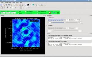
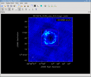
It will take a little while to grid the data, but the viewer will open when it's ready to start an interactive clean. Use the "tape deck" at the bottom of the Viewer display GUI to step through to the channel with the most extended (in angular size) emission, select "all channels" for the clean mask, select the polygon tool (the 'R' with the wobbly line around it) and make a single mask that applies to all channels (see example in thumbnail). Once you make the polygon region, you need to double click inside it to save the mask region -- if you see the polygon turn white you will know you succeeded. Note, that if you had the time and patience you could make a clean mask for each channel, and this would create a slightly better result.
After making the mask you should check that the emission in all the other channels fits within the mask you made using the "tape deck" to move back and forth. If you need to include more area in the mask, you can chose the "erase" toggle at the top, and then encircle your existing mask with a polygon and double click inside. Then go back to "add" toggle at top and make a new mask. Alternatively, you can erase a part of the mask, or you can add to the existing mask by drawing new polygons. Feel free to experiment with this a bit.
Note: If you start an interactive clean, and then do not make a mask, clean will stop when you tell it to go on because it has nothing to clean. There is no default mask.
To continue with clean use the "Next action" buttons in the green area on the Viewer Display GUI: The red X ![]() will stop clean where you are, the blue arrow
will stop clean where you are, the blue arrow ![]() will stop the interactive part of clean, but continue to clean non-interactively until reaching the stopping niter (note that this is "iterations" x "cycles") or threshold (whichever comes first), and the green arrow
will stop the interactive part of clean, but continue to clean non-interactively until reaching the stopping niter (note that this is "iterations" x "cycles") or threshold (whichever comes first), and the green arrow ![]() will clean until it reaches the "iterations" parameter on the left side of the green area. When
the interactive viewer comes back use the tape deck to recheck that your mask encompasses what you think is real emission. The middle mouse button by default controls the image stretch.
will clean until it reaches the "iterations" parameter on the left side of the green area. When
the interactive viewer comes back use the tape deck to recheck that your mask encompasses what you think is real emission. The middle mouse button by default controls the image stretch.
Note that for this example, threshold has been set to threshold = '3mJy' to protect you from cleaning too deeply. With a careful clean mask you can clean to close to the thermal noise limit (note here I mean the actual observed rms noise limit and not the theoretical one you calculated for the proposal, as flagging, weather, etc. can affect what you actually get). It is ALWAYS best to clean each channel in a cube to a specific threshold than to stop by simply using the niter parameter, which can leave each channel cleaned to different levels. There are many ways to determine a suitable threshold. One way is to make a dirty image (niter = 0), open the cube using the viewer, go to a line free channel, select the box region tool, make a box near the field center about the size of your source, and double click inside. The rms noise of that channel will appear in the terminal window from which the viewer was launched. Try a few different boxes, average the results and this is a good estimate of the rms per channel assuming your data are not dynamic range limited (i.e. noise can be higher in channels with strong signal). This is the absolute minimum for threshold. With no mask you probably shouldn't clean deeper than 3x this rms.
Keep cleaning, by using the green Next Action arrow ![]() until the residual displayed in the viewer looks "noise like". To speed things up, you might change the iteration parameter in the viewer to something like 300. This parameter can also be set in the task command. You will notice that in this particular case, there are residuals that cannot be cleaned -- these are due to the extended resolved out structure on size scales larger than the array is sensitive to (the "Largest Angular Scale" or LAS that the array is sensitive to can be calculated from the shortest baseline length), and potential residual phase and amplitude calibration errors. We will explore this in a few sections with self-calibration.
until the residual displayed in the viewer looks "noise like". To speed things up, you might change the iteration parameter in the viewer to something like 300. This parameter can also be set in the task command. You will notice that in this particular case, there are residuals that cannot be cleaned -- these are due to the extended resolved out structure on size scales larger than the array is sensitive to (the "Largest Angular Scale" or LAS that the array is sensitive to can be calculated from the shortest baseline length), and potential residual phase and amplitude calibration errors. We will explore this in a few sections with self-calibration.
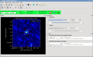
Repeat the process for the SiS line using the call below, note that the emission for this line is less extended than the HC3N -- this has to do with the different excitation requirements of the two different lines. The SiS is excited closer to the central star than the HC3N.
# In CASA
clean(vis='IRC10216.contsub',imagename='IRC10216_SiS.cube_r0.5',
      imagermode='csclean',
      imsize=300,cell=['0.4arcsec'],spw='1:5~58',
      mode='velocity',interpolation='linear',
      restfreq='36.30963GHz',outframe='LSRK',
      weighting='briggs',robust=0.5,
      interactive=T,
      threshold='3.0mJy',niter=100000)
You can look at both cubes using the viewer, and the tape deck to play the cube as a "movie".
# In CASA
viewer
Image the Continuum data
Below the use of mode='mfs' will make a single multi-frequency synthesis image out of the specified spw/channels. Again you should make an interactive clean mask. Since no threshold is set, you will need to stop cleaning when the residual looks noise like using the red x "Next Action" button (it will be done when the viewer comes back the second time). The continuum for IRC10216 is very weak but interesting -- it is essentially tracing the photosphere of the AGB star.
The continuum data set produced with wantcont=True in uvcontsub2 is the model fit. To image the continuum itself, use the line-free channels.
# In CASA
clean(vis='IRC10216',imagename='IRC10216.36GHzcont',
      mode='mfs',imagermode='csclean',
      imsize=300,cell=['0.4arcsec'],spw='0~1:5~14,0~1:48~59',
      weighting='briggs',robust=0.5,
      interactive=T)
Now look at the result in the viewer, if you like:
# In CASA
viewer
Image Analysis and Viewing
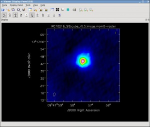
Next make integrated intensity maps (moment 0) and intensity-weighted velocity maps (moment 1). For HC3N, we also produce a velocity dispersion, peak flux, and median map. All are derived with immoments. To do this, we'll want to know what channels the line emission starts and ends on, and also the rms noise in a single channel. So first lets open the viewer:
# In CASA
viewer
Then use the Viewer tape deck to see which channels have significant line emission. For HC3N, the line channel range in the cube is 16 to 45, and it is the same for SiS.
Then use the tape deck to go to a line free channel, select the box region tool and make a box. When you double click in the box, the image statistics for the channel you are on will print to the terminal. Move the box around a bit to see what the variation in rms noise is. You should get something like 2 mJy. Note that the rms is much worse in channels with strong emission because of the low dynamic range of these data. If you want the box tool to go away (i.e. if you want to make a new one), hit the escape key.
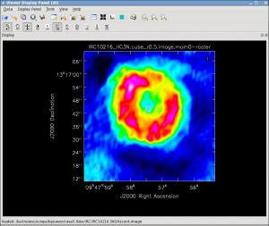
Now let's make the moment 0 and moment 1 maps. For moment zero, it's best to limit the calculation to image channels with significant signal in them, but not to apply a flux cutoff, as this will bias the derived integrated intensities upward.
# In CASA
immoments(imagename='IRC10216_HC3N.cube_r0.5.image',moments=[0],
          axis='spectral',
          chans='16~45',
          outfile='IRC10216_HC3N.cube_r0.5.image.mom0')
# In CASA
immoments(imagename='IRC10216_SiS.cube_r0.5.image',moments=[0],
          axis='spectral',
          chans='16~45',
          outfile='IRC10216_SiS.cube_r0.5.image.mom0')
To have a look at these, use the viewer:
# In CASA
viewer('IRC10216_HC3N.cube_r0.5.image.mom0')
#
viewer('IRC10216_SiS.cube_r0.5.image.mom0')
For moment 1, it is essential to apply a conservative flux cutoff to limit the calculation to high signal-to-noise areas. Here we use about 5σ:
# In CASA
immoments(imagename='IRC10216_HC3N.cube_r0.5.image',moments=[1],
          axis='spectral',
          chans='16~46',excludepix=[-100,0.01],
          outfile='IRC10216_HC3N.cube_r0.5.image.mom1')
# In CASA
immoments(imagename='IRC10216_SiS.cube_r0.5.image',moments=[1],
          axis='spectral',
          chans='16~45',excludepix=[-100,0.01],
          outfile='IRC10216_SiS.cube_r0.5.image.mom1')
Finally, we will do velocity dispersion, peak flux, and median map in a single step for HC3N. immoments can perform these steps even though the latter two are not 'moments' in a mathematical sense. Check the help file to find out the options. Peak flux and median are produced with the moment parameter set to 8 and 3:
# In CASA
immoments(imagename='IRC10216_HC3N.cube_r0.5.image',moments=[2,8,3],
          axis='spectral',
          chans='16~46',excludepix=[-100,0.01],
          outfile='IRC10216_HC3N.cube_r0.5.image.extramoms')
will create the files IRC10216_HC3N.cube_r0.5.image.extramoms.weighted_dispersion_coord, IRC10216_HC3N.cube_r0.5.image.extramoms.median, and IRC10216_HC3N.cube_r0.5.image.extramoms.maximum.
Now use the viewer to further explore the images you've made.
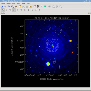
For fun you can download the VLT V-band image at http://casa.nrao.edu/Data/EVLA/IRC10216/irc_fors1_dec_header.fits kindly provided by Izan Leão and overlay the moment images and 36 GHz continuum. More information about the dust properties can be found in the Leão et al. (2006) paper http://adsabs.harvard.edu/abs/2006A%26A...455..187L.
The creation of position velocity cuts from the viewer is currently being developed and hopefully available soon in CASA. If you are interested in a work-around, you may have a look at the pV casaguide. Masking the data cube to extract the emission is described here.
Spectrum Fitting
Frequently, one would like to fit Gaussians or polynomials to the spectral line in the data cube. This can be done with CASA's specfit task. specfit can fit those functions to an average spectrum define by some bounding box, or, alternatively, for each pixel. In the following, we will do both.
Fitting an average spectrum
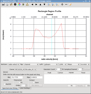
First, we want to inspect the spectrum. Load the image into the viewer (here: the HC3N image cube), select "spectral profile" from the Tools menu and open a region with the mouse button that is assigned to the rectangular "R" region in the tool bar. Best to do this at a plane that shows the entire extent of the source. The average spectrum will be displayed in a separate panel.
To fit this profile in specfit, we need a region file outlining the 2-D region that is averaged (the green box in the viewer screenshot). In the following we use the new CASA region format (CASA 3.3 and higher) that is described here. Following the guidelines on that page, we create a file named specfit.crtf that describes a box with its [[x1,y1],[x2,y2]] corners in J2000 RA DEC coordinates.
#CRTFv0
box[[09:47:59.2, 13.16.24], [09:47:55.8, 13.17.09]]
We will fit 2 Gaussians to the two peaks of the spectrum (the scientific merit is debatable). A file with initial values for the fit can be provided via the estimates parameter - see specfit for details. Here we will let CASA figure out the start values by itself:
# In CASA
myfit = specfit(imagename='IRC10216_HC3N.cube_r0.5.image', region='specfit.crtf', multifit=F,
        estimates='', ngauss=2)
Note that the output is stored in a Python dictionary called "myfit", as well as printed to the CASA logger. You should get something similar to this (depending on the details of flagging etc.):
Fit  :
RA           :   09:47:57.49
Dec          :   13.16.46.46
Stokes       : I
Pixel        : [146.002, 164.499, 0.000,  *]
Attempted    : YES
Converged    : YES
Iterations   : 27
Results for component 0:
    Type     : GAUSSIAN
    Peak     : 6.13 +/- 0.49 mJy/beam
    Center   : -16.34 +/- 0.37 km/s
               40.41 +/- 0.36 pixel
    FWHM     : 8.81 +/- 0.89 km/s
               8.56 +/- 0.87 pixel
    Integral : 57.5 +/- 7.4 mJy/beam.km/s
Results for component 1:
    Type     : GAUSSIAN
    Peak     : 5.40 +/- 0.40 mJy/beam
    Center   : -34.35 +/- 0.51 km/s
               22.92 +/- 0.49 pixel
    FWHM     : 13.4 +/- 1.3 km/s
               13.0 +/- 1.3 pixel
    Integral : 77.2 +/- 9.4 mJy/beam.km/s
which seems to have caught the two peaks pretty well.
Spectral Fitting pixel by pixel
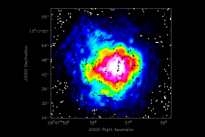
specfit can also fit Gaussians to every spectrum in each single spatial pixel. The following command will do this within the spectfit.crtf region defined above:
# In CASA
pixfit = specfit(imagename='IRC10216_HC3N.cube_r0.5.image', region='specfit.crtf', ngauss=2,
         multifit=T,  amp='fit.amp.image', center='fitcenter.image', fwhm='fitfwhm.image')
In this example, specfit will produce three images per Gaussian, images that map the best fit values of the Gauss peaks (amplitudes), velocity centers, and full widths at half maximum. For the first Gaussian, the image to the right displays the amplitude image fit.amp.image_0.
Self-Calibration
The many different aspects of self-calibration could fill several casaguides. Here we describe a simple process for this particular relatively low S/N data (low S/N per channel, at least).
While running clean above, the model column for each channel will have been filled with the clean model (if you made a Fourier transform of this model, you would see an image of the clean components).
We choose to do the self cal on the spw=1 SiS line data because it has the strongest emission in a single channel and is a bit more compact than the HC3N data. We will run gaincal specifying the channel in the uv-data that has the brightest peak in the image (use the viewer to figure out which channel this is for spw=1), note down what the peak flux is. Since we started the image with a channel range we need to account for the fact that the image channel numbers do not map exactly to the uv-data channel numbers (they are off by 5 so that channel 13 in the image is roughly channel 19 in the uv-data).
The next thing we need to understand is the S/N of the data. In particular, to self-cal, you need enough signal on a single baseline over the course of your chosen solint to get a S/N of about 3. Above we calculated an average rms noise of about 2 mJy/beam/channel for the whole timerange (about 95 minutes on source time) and all antennas (16). We can use our knowledge of the radiometer equation (see EVLA Sensitivity) where rms scales as 1/sqrt(time * #baselines), and the number of baselines= N(N-1)/2 and N=# of antennas. So the rms noise on one baseline, for one 10 second integration in this observation is given by:
[math]\displaystyle{ {\rm RMS(baseline)} = {\rm 2\ mJy\ beam^{-1}\ channel^{-1}} \sqrt{ \frac{95\times 60\ {\rm sec}}{10\ {\rm sec}}\times\frac{16\times 15}{2\times 1}}\ {\sim}\ 500\ {\rm mJy\ beam^{-1}\ channel^{-1}} }[/math]
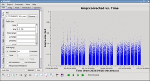
The 95 minutes of on-source time can be estimated from a plot like this where you can sum up the amount of time on a source:
# In CASA
plotms(vis='day2_TDEM0003_10s_norx',field='3',ydatacolumn='corrected',
       xaxis='time',yaxis='amp',correlation='RR,LL',
       avgchannel='64',spw='1:4~60',antenna='')
This analysis suggests that the rms noise on one baseline, for one 10 second integration is only about 500 mJy. In contrast, the peak flux density in the strongest SiS channel is only about 200 mJy (you can check using the viewer). Since the emission is fairly compact, most baselines will see about this peak flux; this is why we choose the more compact of the two possible lines. Thus, a 10 second solution interval is not enough to get a SNR of at least 3 on a 200 mJy peak. We need to use a solint large enough so that the rms noise is not worse than about 1/3 of 200 mJy. Thus, a solint of 10 minutes is about the shortest we can use and be reasonably confident of the solutions.
Now we run gaincal with the solint we have determined. Note that because our desired solint is more than the scan time, we need to include combine='scan'.
# In CASA
gaincal(vis='IRC10216.contsub',caltable='pcal_ch19one_10min',
        spw='1:19~19',calmode='p',solint='10min',combine='scan',
        refant='ea02',minsnr=3.0)
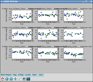
Now let's look at the solutions:
# In CASA
plotcal(caltable='pcal_ch19one_10min',xaxis='time',yaxis='phase',
        iteration='antenna',subplot=331,plotrange=[0,0,-50,50])
For some antennas you can see clear global trends away from zero: ea08, ea21, and ea24 are examples, and you can also see some smaller variations with time.
Now let's explore whether applying this solution actually improves matters. To do this we need to run applycal to apply the solutions to the line dataset, both spw. We need to use spwmap to tell it that the solutions derived for spw=1 should be applied to both spw=0 and spw=1. Again it's important to set calwt=F here.
# In CASA
applycal(vis='IRC10216.contsub',field='',spw='0,1',
        gaintable=['pcal_ch19one_10min'],spwmap=[[1,1]],calwt=F)
Note: in this example we ran the self-cal steps on the full uv continuum subtracted spectral line data set. For a more complex iterative self-calibration proceedure, you may find it easier to split off the channel/spw you want to experiment on with split, and then do all the imaging (clean) and gaincal steps with it. The gaincal tables created on the single channel can still be applied with applycal to the multi-channel/spw dataset. If you do this though, keep in mind that once split, the single-channel data will have its spw id reset to 0 (you can check with listobs), no matter what spw it came from. Thus in order to applycal with it you would need spwmap=[[0,0]].
To save time we can use the clean mask we made before and run in a non-interactive mode. You can use a mask over again as long as the number of channels in the clean call haven't changed. You can change cell or imsize and it will still do the right thing.
# In CASA
clean(vis='IRC10216.contsub',imagename='IRC10216_HC3N.cube_r0.5.pselfcal',
      imagermode='csclean',
      imsize=300,cell=['0.4arcsec'],spw='0:5~58',
      mode='velocity',interpolation='linear',
      restfreq='36.39232GHz',outframe='LSRK',
      weighting='briggs',robust=0.5,
      mask='IRC10216_HC3N.cube_r0.5.mask',
      interactive=F,threshold='3.0mJy',niter=100000)
# In CASA
clean(vis='IRC10216.contsub',imagename='IRC10216_SiS.cube_r0.5.pselfcal',
      imagermode='csclean',calready=T,
      imsize=300,cell=['0.4arcsec'],spw='1:5~58',
      mode='velocity',interpolation='linear',
      restfreq='36.30963GHz',outframe='LSRK',
      weighting='briggs',robust=0.5,
      mask='IRC10216_SiS.cube_r0.5.mask',
      interactive=F,threshold='3.0mJy',niter=100000)
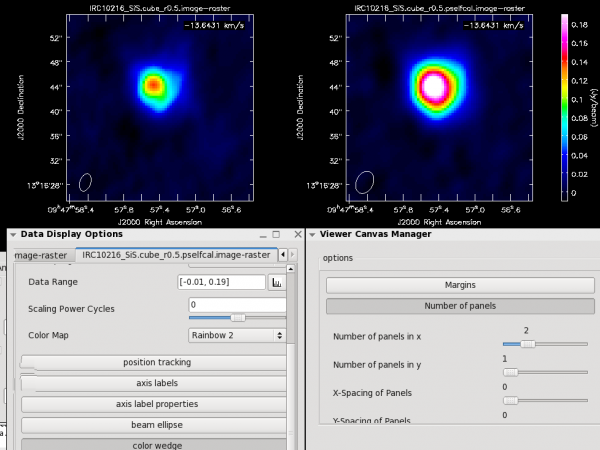
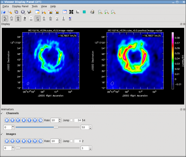
Now investigate the original and self-cal'ed images in the viewer. You will find that even this single self-cal step significantly improves the images. Try opening both versions of the SiS image cubes. Then select a bright channel from the tape deck like channel 37, then use the "wrench" and "pwrench" guis to make a plot like below setting the same image range for both cubes, and two panels in x, then to see both images of that channel side-by-side click the blink toggle (see image below for more tips on setup.)
Repeat for HC3N:
Now you can redo the moment images if you like with the improved cubes (be sure to change the output file). names.
--Crystal Brogan --additions:Juergen Ott, Miriam Krauss
Last checked on CASA Version 3.3.0.
