EVLA 3-bit Tutorial G192-CASA4.4
This is an advanced Jansky VLA data reduction tutorial that calibrates and images a 3-bit dataset.
This CASA Guide is for CASA version 4.4
Overview
This article describes the calibration and imaging of the protostar G192.16-3.84. The data were taken in Ka-band using the VLA's 3-bit samplers and widely-spaced basebands centered at 29 and 36.5 GHz. Each baseband has over 4 GHz of bandwidth comprised of 32 128-MHz spectral windows. In this tutorial, we will examine, flag, and calibrate the data, including the corrections for the requantizer gains (which are necessary for 3-bit data calibration and harmless on 8-bit data). We will then image and analyze the calibrated data, using wideband imaging techniques.
This is a more advanced tutorial, so if you are a relative novice, it is strongly recommended that you start with the EVLA Continuum Tutorial 3C391 (at least read it through) before proceeding with this tutorial.
In addition, on the MainPage of the CASA Guides you can find these helpful pages:
- What is CASA?
- Getting Started in CASA
- CASA Reference Manuals
- Hints, Tips, & Tricks
- AIPS-to-CASA Cheat Sheet
In this tutorial we will be invoking the tasks as function calls. You can cut and paste these to your casapy session. We also recommend that you copy all the commands you use, with any relevant commentary, to a text file. This is very good practice when tackling large datasets. If you wish, you can use the Script Extractor to create a file with the tutorial commands, which can subsequently be edited and annotated as desired.
Occasionally we will be setting Python variables (e.g., as lists for flags) outside the function call so make sure you set those before running the task command. Note that when you call a CASA task as a function, any task parameters that are not set in the function call will be used with their default values. This means they will not use values you set in any previous calls or outside the call. See Getting_Started_in_CASA#Task_Execution for more on calling tasks and setting parameters in the scripting interface.
NOTE: If you find that the figures on the right margin of the browser window overlap the text too much and make reading difficult, you can adjust the width of the browser window.
Obtaining the Data
The data for this tutorial were taken with the VLA during its commissioning phase. They comprise the scheduling block (SB) TVER0004.sb14459364.eb14492359.56295.26287841435, which was run on 2013-01-03 from 6:18 to 7:47 UT (its raw size is 57.04 GB).
The data can be downloaded directly from http://casa.nrao.edu/Data/EVLA/G192/G192_6s.ms.tar.gz (dataset size: 18 GB)
Your first step will be to unzip and untar the file in a terminal (before you start CASA):
tar -xzvf G192_6s.ms.tar.gz
If you are brave enough, you can also get the data directly from the VLA archive. Go to the NRAO Science Data Archive, and search for "TVER0004.sb14459364" in the Archive File ID field. Then select the dataset and choose a time-averaging value of 6 seconds. (Although the data were taken in A-configuration, we will not be imaging outside of the center of the field, so we aren't too worried about time-average smearing and will take advantage of averaging to reduce the dataset size.) Also select the "Create tar file" option.
In addition, only the fields used for analysis and observation are included in the downloadable file. This can be accomplished using the split task in CASA:
# In CASA: splitting fields for analysis
split('TVER0004.sb14459364.eb14492359.56295.26287841435.ms', outputvis='G192_6s.ms', \
      datacolumn='all', field='3,6,7,10', keepflags=False, spw='2~65')
(If you're downloading from the archive and feeling ambitious, you could also select only the scans with fields 3, 6, 7, and 10 in the "Select scans for MS or AIPS FITS" box.) This will create a file equivalent to what is used at the start of this tutorial.
Finally, you will need to modify some information in the SOURCE and FIELD tables of the measurement set (this has already been done for you in the file available for download, but must be done by hand if obtaining from the archive). Follow the instructions here to make these changes.
Starting CASA
To start CASA, type:
casa
This will run a script to initialize CASA, setting paths appropriately. It will also start writing to a file called ipython-<unique-stamp>.log, which will contain a record of all the text you enter at the CASA prompt, as well as casapy-<unique-stamp>.log, which will contain all the messages that are printed to the CASA logger window. It is recommended that you keep your log files in tact - you may need them to remind you of the last step you completed in your data reduction! (It is also a good idea to include your log files when submitting a help desk ticket).
Once CASA has started, a logger window will appear. Note that you can rescale this window or change the font size as desired (the latter is under "View").
Examining the Measurement Set (MS)
We use listobs to summarize our MS:
# In CASA: listobs on the initial data set
listobs('G192_6s.ms', listfile='G192_listobs.txt')
This will write the output to a file called G192_listobs.txt, which we can print to the terminal using the cat command:
# In CASA
cat G192_listobs.txt
##########################################
##### Begin Task: listobs #####
listobs(vis="G192_6s.ms",selectdata=True,spw="",field="",antenna="",
uvrange="",timerange="",correlation="",scan="",intent="",
feed="",array="",observation="",verbose=True,listfile="",
listunfl=False,cachesize=50,overwrite=False)
================================================================================
MeasurementSet Name: /export/home/sledgehammer2/jott/casatest/G192/G192_6s.ms MS Version 2
================================================================================
Observer: Dr. Debra Shepherd Project: uid://evla/pdb/7303457
Observation: EVLA
Data records: 10061248 Total elapsed time = 4563 seconds
Observed from 03-Jan-2013/06:31:48.0 to 03-Jan-2013/07:47:51.0 (UTC)
ObservationID = 0 ArrayID = 0
Date Timerange (UTC) Scan FldId FieldName nRows SpwIds Average Interval(s) ScanIntent
03-Jan-2013/06:31:48.0 - 06:36:42.0 6 0 3C147 1019200 [0,1,2,3,4,5,6,7,8,9,10,11,12,13,14,15,16,17,18,19,20,21,22,23,24,25,26,27,28,29,30,31,32,33,34,35,36,37,38,39,40,41,42,43,44,45,46,47,48,49,50,51,52,53,54,55,56,57,58,59,60,61,62,63] [6, 6, 6, 6, 6, 6, 6, 6, 6, 6, 6, 6, 6, 6, 6, 6, 6, 6, 6, 6, 6, 6, 6, 6, 6, 6, 6, 6, 6, 5.94, 6, 6, 6, 6, 6, 6, 6, 6, 6, 6, 6, 6, 6, 6, 6, 6, 6, 6, 6, 6, 6, 6, 6, 6, 6, 6, 6, 6, 6, 6, 6, 6, 6, 6] [CALIBRATE_FLUX#UNSPECIFIED,OBSERVE_TARGET#UNSPECIFIED]
06:46:15.0 - 06:46:54.0 10 1 gcal-J0603+174 145600 [0,1,2,3,4,5,6,7,8,9,10,11,12,13,14,15,16,17,18,19,20,21,22,23,24,25,26,27,28,29,30,31,32,33,34,35,36,37,38,39,40,41,42,43,44,45,46,47,48,49,50,51,52,53,54,55,56,57,58,59,60,61,62,63] [5.57, 5.57, 5.57, 5.57, 5.57, 5.57, 5.57, 5.57, 5.57, 5.57, 5.57, 5.57, 5.57, 5.57, 5.57, 5.57, 5.57, 5.57, 5.57, 5.57, 5.57, 5.57, 5.57, 5.57, 5.57, 5.57, 5.57, 5.57, 5.57, 5.57, 5.57, 5.57, 5.57, 5.57, 5.57, 5.57, 5.57, 5.57, 5.57, 5.57, 5.57, 5.57, 5.57, 5.57, 5.57, 5.57, 5.57, 5.57, 5.57, 5.57, 5.57, 5.57, 5.57, 5.57, 5.57, 5.57, 5.57, 5.57, 5.57, 5.57, 5.57, 5.57, 5.57, 5.57] [CALIBRATE_AMPLI#UNSPECIFIED,CALIBRATE_PHASE#UNSPECIFIED,OBSERVE_TARGET#UNSPECIFIED]
06:47:09.0 - 06:47:54.0 11 2 G192.16-3.84 163200 [0,1,2,3,4,5,6,7,8,9,10,11,12,13,14,15,16,17,18,19,20,21,22,23,24,25,26,27,28,29,30,31,32,33,34,35,36,37,38,39,40,41,42,43,44,45,46,47,48,49,50,51,52,53,54,55,56,57,58,59,60,61,62,63] [5.65, 5.65, 5.65, 5.65, 5.65, 5.65, 5.65, 5.65, 5.65, 5.65, 5.65, 5.65, 5.65, 5.65, 5.65, 5.65, 5.65, 5.65, 5.65, 5.65, 5.65, 5.65, 5.65, 5.65, 5.65, 5.65, 5.65, 5.65, 5.65, 5.65, 5.65, 5.65, 5.65, 5.65, 5.65, 5.65, 5.65, 5.65, 5.65, 5.65, 5.65, 5.65, 5.65, 5.65, 5.65, 5.65, 5.65, 5.65, 5.65, 5.65, 5.65, 5.65, 5.65, 5.65, 5.65, 5.65, 5.65, 5.65, 5.65, 5.65, 5.65, 5.65, 5.65, 5.65] [OBSERVE_TARGET#UNSPECIFIED]
06:48:06.0 - 06:48:39.0 12 1 gcal-J0603+174 124800 [0,1,2,3,4,5,6,7,8,9,10,11,12,13,14,15,16,17,18,19,20,21,22,23,24,25,26,27,28,29,30,31,32,33,34,35,36,37,38,39,40,41,42,43,44,45,46,47,48,49,50,51,52,53,54,55,56,57,58,59,60,61,62,63] [5.5, 5.5, 5.5, 5.5, 5.5, 5.5, 5.5, 5.5, 5.5, 5.5, 5.5, 5.5, 5.5, 5.5, 5.5, 5.5, 5.5, 5.5, 5.5, 5.5, 5.5, 5.5, 5.5, 5.5, 5.5, 5.5, 5.5, 5.5, 5.5, 5.5, 5.5, 5.5, 5.5, 5.5, 5.5, 5.5, 5.5, 5.5, 5.5, 5.5, 5.5, 5.5, 5.5, 5.5, 5.5, 5.5, 5.5, 5.5, 5.5, 5.5, 5.5, 5.5, 5.5, 5.5, 5.5, 5.5, 5.5, 5.5, 5.5, 5.5, 5.5, 5.5, 5.5, 5.5] [CALIBRATE_AMPLI#UNSPECIFIED,CALIBRATE_PHASE#UNSPECIFIED,OBSERVE_TARGET#UNSPECIFIED]
06:48:51.0 - 06:49:39.0 13 2 G192.16-3.84 166400 [0,1,2,3,4,5,6,7,8,9,10,11,12,13,14,15,16,17,18,19,20,21,22,23,24,25,26,27,28,29,30,31,32,33,34,35,36,37,38,39,40,41,42,43,44,45,46,47,48,49,50,51,52,53,54,55,56,57,58,59,60,61,62,63] [6, 6, 6, 6, 6, 6, 6, 6, 6, 6, 6, 6, 6, 6, 6, 6, 6, 6, 6, 6, 6, 6, 6, 6, 6, 6, 6, 6, 6, 6, 6, 6, 6, 6, 6, 6, 6, 6, 6, 6, 6, 6, 6, 6, 6, 6, 6, 6, 6, 6, 6, 6, 6, 6, 6, 6, 6, 6, 6, 6, 6, 6, 6, 6] [OBSERVE_TARGET#UNSPECIFIED]
06:49:51.0 - 06:50:24.0 14 1 gcal-J0603+174 124800 [0,1,2,3,4,5,6,7,8,9,10,11,12,13,14,15,16,17,18,19,20,21,22,23,24,25,26,27,28,29,30,31,32,33,34,35,36,37,38,39,40,41,42,43,44,45,46,47,48,49,50,51,52,53,54,55,56,57,58,59,60,61,62,63] [5.5, 5.5, 5.5, 5.5, 5.5, 5.5, 5.5, 5.5, 5.5, 5.5, 5.5, 5.5, 5.5, 5.5, 5.5, 5.5, 5.5, 5.5, 5.5, 5.5, 5.5, 5.5, 5.5, 5.5, 5.5, 5.5, 5.5, 5.5, 5.5, 5.5, 5.5, 5.5, 5.5, 5.5, 5.5, 5.5, 5.5, 5.5, 5.5, 5.5, 5.5, 5.5, 5.5, 5.5, 5.5, 5.5, 5.5, 5.5, 5.5, 5.5, 5.5, 5.5, 5.5, 5.5, 5.5, 5.5, 5.5, 5.5, 5.5, 5.5, 5.5, 5.5, 5.5, 5.5] [CALIBRATE_AMPLI#UNSPECIFIED,CALIBRATE_PHASE#UNSPECIFIED,OBSERVE_TARGET#UNSPECIFIED]
06:50:36.0 - 06:51:24.0 15 2 G192.16-3.84 166400 [0,1,2,3,4,5,6,7,8,9,10,11,12,13,14,15,16,17,18,19,20,21,22,23,24,25,26,27,28,29,30,31,32,33,34,35,36,37,38,39,40,41,42,43,44,45,46,47,48,49,50,51,52,53,54,55,56,57,58,59,60,61,62,63] [6, 6, 6, 6, 6, 6, 6, 6, 6, 6, 6, 6, 6, 6, 6, 6, 6, 6, 6, 6, 6, 6, 6, 6, 6, 6, 6, 6, 6, 6, 6, 6, 6, 6, 6, 6, 6, 6, 6, 6, 6, 6, 6, 6, 6, 6, 6, 6, 6, 6, 6, 6, 6, 6, 6, 6, 6, 6, 6, 6, 6, 6, 6, 6] [OBSERVE_TARGET#UNSPECIFIED]
06:51:36.0 - 06:52:09.0 16 1 gcal-J0603+174 124800 [0,1,2,3,4,5,6,7,8,9,10,11,12,13,14,15,16,17,18,19,20,21,22,23,24,25,26,27,28,29,30,31,32,33,34,35,36,37,38,39,40,41,42,43,44,45,46,47,48,49,50,51,52,53,54,55,56,57,58,59,60,61,62,63] [5.5, 5.5, 5.5, 5.5, 5.5, 5.5, 5.5, 5.5, 5.5, 5.5, 5.5, 5.5, 5.5, 5.5, 5.5, 5.5, 5.5, 5.5, 5.5, 5.5, 5.5, 5.5, 5.5, 5.5, 5.5, 5.5, 5.5, 5.5, 5.5, 5.5, 5.5, 5.5, 5.5, 5.5, 5.5, 5.5, 5.5, 5.5, 5.5, 5.5, 5.5, 5.5, 5.5, 5.5, 5.5, 5.5, 5.5, 5.5, 5.5, 5.5, 5.5, 5.5, 5.5, 5.5, 5.5, 5.5, 5.5, 5.5, 5.5, 5.5, 5.5, 5.5, 5.5, 5.5] [CALIBRATE_AMPLI#UNSPECIFIED,CALIBRATE_PHASE#UNSPECIFIED,OBSERVE_TARGET#UNSPECIFIED]
06:52:21.0 - 06:53:09.0 17 2 G192.16-3.84 166400 [0,1,2,3,4,5,6,7,8,9,10,11,12,13,14,15,16,17,18,19,20,21,22,23,24,25,26,27,28,29,30,31,32,33,34,35,36,37,38,39,40,41,42,43,44,45,46,47,48,49,50,51,52,53,54,55,56,57,58,59,60,61,62,63] [6, 6, 6, 6, 6, 6, 6, 6, 6, 6, 6, 6, 6, 6, 6, 6, 6, 6, 6, 6, 6, 6, 6, 6, 6, 6, 6, 6, 6, 6, 6, 6, 6, 6, 6, 6, 6, 6, 6, 6, 6, 6, 6, 6, 6, 6, 6, 6, 6, 6, 6, 6, 6, 6, 6, 6, 6, 6, 6, 6, 6, 6, 6, 6] [OBSERVE_TARGET#UNSPECIFIED]
06:53:21.0 - 06:53:54.0 18 1 gcal-J0603+174 124800 [0,1,2,3,4,5,6,7,8,9,10,11,12,13,14,15,16,17,18,19,20,21,22,23,24,25,26,27,28,29,30,31,32,33,34,35,36,37,38,39,40,41,42,43,44,45,46,47,48,49,50,51,52,53,54,55,56,57,58,59,60,61,62,63] [5.5, 5.5, 5.5, 5.5, 5.5, 5.5, 5.5, 5.5, 5.5, 5.5, 5.5, 5.5, 5.5, 5.5, 5.5, 5.5, 5.5, 5.5, 5.5, 5.5, 5.5, 5.5, 5.5, 5.5, 5.5, 5.5, 5.5, 5.5, 5.5, 5.5, 5.5, 5.5, 5.5, 5.5, 5.5, 5.5, 5.5, 5.5, 5.5, 5.5, 5.5, 5.5, 5.5, 5.5, 5.5, 5.5, 5.5, 5.5, 5.5, 5.5, 5.5, 5.5, 5.5, 5.5, 5.5, 5.5, 5.5, 5.5, 5.5, 5.5, 5.5, 5.5, 5.5, 5.5] [CALIBRATE_AMPLI#UNSPECIFIED,CALIBRATE_PHASE#UNSPECIFIED,OBSERVE_TARGET#UNSPECIFIED]
06:54:06.0 - 06:54:54.0 19 2 G192.16-3.84 166400 [0,1,2,3,4,5,6,7,8,9,10,11,12,13,14,15,16,17,18,19,20,21,22,23,24,25,26,27,28,29,30,31,32,33,34,35,36,37,38,39,40,41,42,43,44,45,46,47,48,49,50,51,52,53,54,55,56,57,58,59,60,61,62,63] [6, 6, 6, 6, 6, 6, 6, 6, 6, 6, 6, 6, 6, 6, 6, 6, 6, 6, 6, 6, 6, 6, 6, 6, 6, 6, 6, 6, 6, 6, 6, 6, 6, 6, 6, 6, 6, 6, 6, 6, 6, 6, 6, 6, 6, 6, 6, 6, 6, 6, 6, 6, 6, 6, 6, 6, 6, 6, 6, 6, 6, 6, 6, 6] [OBSERVE_TARGET#UNSPECIFIED]
06:55:06.0 - 06:55:39.0 20 1 gcal-J0603+174 124800 [0,1,2,3,4,5,6,7,8,9,10,11,12,13,14,15,16,17,18,19,20,21,22,23,24,25,26,27,28,29,30,31,32,33,34,35,36,37,38,39,40,41,42,43,44,45,46,47,48,49,50,51,52,53,54,55,56,57,58,59,60,61,62,63] [5.5, 5.5, 5.5, 5.5, 5.5, 5.5, 5.5, 5.5, 5.5, 5.5, 5.5, 5.5, 5.5, 5.5, 5.5, 5.5, 5.5, 5.5, 5.5, 5.5, 5.5, 5.5, 5.5, 5.5, 5.5, 5.5, 5.5, 5.5, 5.5, 5.5, 5.5, 5.5, 5.5, 5.5, 5.5, 5.5, 5.5, 5.5, 5.5, 5.5, 5.5, 5.5, 5.5, 5.5, 5.5, 5.5, 5.5, 5.5, 5.5, 5.5, 5.5, 5.5, 5.5, 5.5, 5.5, 5.5, 5.5, 5.5, 5.5, 5.5, 5.5, 5.5, 5.5, 5.5] [CALIBRATE_AMPLI#UNSPECIFIED,CALIBRATE_PHASE#UNSPECIFIED,OBSERVE_TARGET#UNSPECIFIED]
06:55:51.0 - 06:56:39.0 21 2 G192.16-3.84 166400 [0,1,2,3,4,5,6,7,8,9,10,11,12,13,14,15,16,17,18,19,20,21,22,23,24,25,26,27,28,29,30,31,32,33,34,35,36,37,38,39,40,41,42,43,44,45,46,47,48,49,50,51,52,53,54,55,56,57,58,59,60,61,62,63] [6, 6, 6, 6, 6, 6, 6, 6, 6, 6, 6, 6, 6, 6, 6, 6, 6, 6, 6, 6, 6, 6, 6, 6, 6, 6, 6, 6, 6, 6, 6, 6, 6, 6, 6, 6, 6, 6, 6, 6, 6, 6, 6, 6, 6, 6, 6, 6, 6, 6, 6, 6, 6, 6, 6, 6, 6, 6, 6, 6, 6, 6, 6, 6] [OBSERVE_TARGET#UNSPECIFIED]
06:56:51.0 - 06:57:24.0 22 1 gcal-J0603+174 124800 [0,1,2,3,4,5,6,7,8,9,10,11,12,13,14,15,16,17,18,19,20,21,22,23,24,25,26,27,28,29,30,31,32,33,34,35,36,37,38,39,40,41,42,43,44,45,46,47,48,49,50,51,52,53,54,55,56,57,58,59,60,61,62,63] [5.5, 5.5, 5.5, 5.5, 5.5, 5.5, 5.5, 5.5, 5.5, 5.5, 5.5, 5.5, 5.5, 5.5, 5.5, 5.5, 5.5, 5.5, 5.5, 5.5, 5.5, 5.5, 5.5, 5.5, 5.5, 5.5, 5.5, 5.5, 5.5, 5.5, 5.5, 5.5, 5.5, 5.5, 5.5, 5.5, 5.5, 5.5, 5.5, 5.5, 5.5, 5.5, 5.5, 5.5, 5.5, 5.5, 5.5, 5.5, 5.5, 5.5, 5.5, 5.5, 5.5, 5.5, 5.5, 5.5, 5.5, 5.5, 5.5, 5.5, 5.5, 5.5, 5.5, 5.5] [CALIBRATE_AMPLI#UNSPECIFIED,CALIBRATE_PHASE#UNSPECIFIED,OBSERVE_TARGET#UNSPECIFIED]
06:57:36.0 - 06:58:24.0 23 2 G192.16-3.84 166400 [0,1,2,3,4,5,6,7,8,9,10,11,12,13,14,15,16,17,18,19,20,21,22,23,24,25,26,27,28,29,30,31,32,33,34,35,36,37,38,39,40,41,42,43,44,45,46,47,48,49,50,51,52,53,54,55,56,57,58,59,60,61,62,63] [6, 6, 6, 6, 6, 6, 6, 6, 6, 6, 6, 6, 6, 6, 6, 6, 6, 6, 6, 6, 6, 6, 6, 6, 6, 6, 6, 6, 6, 6, 6, 6, 6, 6, 6, 6, 6, 6, 6, 6, 6, 6, 6, 6, 6, 6, 6, 6, 6, 6, 6, 6, 6, 6, 6, 6, 6, 6, 6, 6, 6, 6, 6, 6] [OBSERVE_TARGET#UNSPECIFIED]
06:58:36.0 - 06:59:12.0 24 1 gcal-J0603+174 124800 [0,1,2,3,4,5,6,7,8,9,10,11,12,13,14,15,16,17,18,19,20,21,22,23,24,25,26,27,28,29,30,31,32,33,34,35,36,37,38,39,40,41,42,43,44,45,46,47,48,49,50,51,52,53,54,55,56,57,58,59,60,61,62,63] [6, 6, 6, 6, 6, 6, 6, 6, 6, 6, 6, 6, 6, 6, 6, 6, 6, 6, 6, 6, 6, 6, 6, 6, 6, 6, 6, 6, 6, 6, 6, 6, 6, 6, 6, 6, 6, 6, 6, 6, 6, 6, 6, 6, 6, 6, 6, 6, 6, 6, 6, 6, 6, 6, 6, 6, 6, 6, 6, 6, 6, 6, 6, 6] [CALIBRATE_AMPLI#UNSPECIFIED,CALIBRATE_PHASE#UNSPECIFIED,OBSERVE_TARGET#UNSPECIFIED]
06:59:21.0 - 07:00:12.0 25 2 G192.16-3.84 187200 [0,1,2,3,4,5,6,7,8,9,10,11,12,13,14,15,16,17,18,19,20,21,22,23,24,25,26,27,28,29,30,31,32,33,34,35,36,37,38,39,40,41,42,43,44,45,46,47,48,49,50,51,52,53,54,55,56,57,58,59,60,61,62,63] [5.67, 5.67, 5.67, 5.67, 5.67, 5.67, 5.67, 5.67, 5.67, 5.67, 5.67, 5.67, 5.67, 5.67, 5.67, 5.67, 5.67, 5.67, 5.67, 5.67, 5.67, 5.67, 5.67, 5.67, 5.67, 5.67, 5.67, 5.67, 5.67, 5.67, 5.67, 5.67, 5.67, 5.67, 5.67, 5.67, 5.67, 5.67, 5.67, 5.67, 5.67, 5.67, 5.67, 5.67, 5.67, 5.67, 5.67, 5.67, 5.67, 5.67, 5.67, 5.67, 5.67, 5.67, 5.67, 5.67, 5.67, 5.67, 5.67, 5.67, 5.67, 5.67, 5.67, 5.67] [OBSERVE_TARGET#UNSPECIFIED]
07:00:21.0 - 07:00:57.0 26 1 gcal-J0603+174 124800 [0,1,2,3,4,5,6,7,8,9,10,11,12,13,14,15,16,17,18,19,20,21,22,23,24,25,26,27,28,29,30,31,32,33,34,35,36,37,38,39,40,41,42,43,44,45,46,47,48,49,50,51,52,53,54,55,56,57,58,59,60,61,62,63] [6, 6, 6, 6, 6, 6, 6, 6, 6, 6, 6, 6, 6, 6, 6, 6, 6, 6, 6, 6, 6, 6, 6, 6, 6, 6, 6, 6, 6, 6, 6, 6, 6, 6, 6, 6, 6, 6, 6, 6, 6, 6, 6, 6, 6, 6, 6, 6, 6, 6, 6, 6, 6, 6, 6, 6, 6, 6, 6, 6, 6, 6, 6, 6] [CALIBRATE_AMPLI#UNSPECIFIED,CALIBRATE_PHASE#UNSPECIFIED,OBSERVE_TARGET#UNSPECIFIED]
07:01:06.0 - 07:01:57.0 27 2 G192.16-3.84 187200 [0,1,2,3,4,5,6,7,8,9,10,11,12,13,14,15,16,17,18,19,20,21,22,23,24,25,26,27,28,29,30,31,32,33,34,35,36,37,38,39,40,41,42,43,44,45,46,47,48,49,50,51,52,53,54,55,56,57,58,59,60,61,62,63] [5.67, 5.67, 5.67, 5.67, 5.67, 5.67, 5.67, 5.67, 5.67, 5.67, 5.67, 5.67, 5.67, 5.67, 5.67, 5.67, 5.67, 5.67, 5.67, 5.67, 5.67, 5.67, 5.67, 5.67, 5.67, 5.67, 5.67, 5.67, 5.67, 5.67, 5.67, 5.67, 5.67, 5.67, 5.67, 5.67, 5.67, 5.67, 5.67, 5.67, 5.67, 5.67, 5.67, 5.67, 5.67, 5.67, 5.67, 5.67, 5.67, 5.67, 5.67, 5.67, 5.67, 5.67, 5.67, 5.67, 5.67, 5.67, 5.67, 5.67, 5.67, 5.67, 5.67, 5.67] [OBSERVE_TARGET#UNSPECIFIED]
07:02:03.0 - 07:02:42.0 28 1 gcal-J0603+174 125184 [0,1,2,3,4,5,6,7,8,9,10,11,12,13,14,15,16,17,18,19,20,21,22,23,24,25,26,27,28,29,30,31,32,33,34,35,36,37,38,39,40,41,42,43,44,45,46,47,48,49,50,51,52,53,54,55,56,57,58,59,60,61,62,63] [5.99, 5.99, 5.99, 5.99, 5.99, 5.99, 5.99, 5.99, 5.99, 5.99, 5.99, 5.99, 5.99, 5.99, 5.99, 5.99, 5.99, 5.99, 5.99, 5.99, 5.99, 5.99, 5.99, 5.99, 5.99, 5.99, 5.99, 5.99, 5.99, 5.99, 5.99, 5.99, 5.99, 5.99, 5.99, 5.99, 5.99, 5.99, 5.99, 5.99, 5.99, 5.99, 5.99, 5.99, 5.99, 5.99, 5.99, 5.99, 5.99, 5.99, 5.99, 5.99, 5.99, 5.99, 5.99, 5.99, 5.99, 5.99, 5.99, 5.99, 5.99, 5.99, 5.99, 5.99] [CALIBRATE_AMPLI#UNSPECIFIED,CALIBRATE_PHASE#UNSPECIFIED,OBSERVE_TARGET#UNSPECIFIED]
07:02:48.0 - 07:03:36.0 29 2 G192.16-3.84 166400 [0,1,2,3,4,5,6,7,8,9,10,11,12,13,14,15,16,17,18,19,20,21,22,23,24,25,26,27,28,29,30,31,32,33,34,35,36,37,38,39,40,41,42,43,44,45,46,47,48,49,50,51,52,53,54,55,56,57,58,59,60,61,62,63] [6, 6, 6, 6, 6, 6, 6, 6, 6, 6, 6, 6, 6, 6, 6, 6, 6, 6, 6, 6, 6, 6, 6, 6, 6, 6, 6, 6, 6, 6, 6, 6, 6, 6, 6, 6, 6, 6, 6, 6, 6, 6, 6, 6, 6, 6, 6, 6, 6, 6, 6, 6, 6, 6, 6, 6, 6, 6, 6, 6, 6, 6, 6, 6] [OBSERVE_TARGET#UNSPECIFIED]
07:03:48.0 - 07:04:21.0 30 1 gcal-J0603+174 124800 [0,1,2,3,4,5,6,7,8,9,10,11,12,13,14,15,16,17,18,19,20,21,22,23,24,25,26,27,28,29,30,31,32,33,34,35,36,37,38,39,40,41,42,43,44,45,46,47,48,49,50,51,52,53,54,55,56,57,58,59,60,61,62,63] [5.5, 5.5, 5.5, 5.5, 5.5, 5.5, 5.5, 5.5, 5.5, 5.5, 5.5, 5.5, 5.5, 5.5, 5.5, 5.5, 5.5, 5.5, 5.5, 5.5, 5.5, 5.5, 5.5, 5.5, 5.5, 5.5, 5.5, 5.5, 5.5, 5.5, 5.5, 5.5, 5.5, 5.5, 5.5, 5.5, 5.5, 5.5, 5.5, 5.5, 5.5, 5.5, 5.5, 5.5, 5.5, 5.5, 5.5, 5.5, 5.5, 5.5, 5.5, 5.5, 5.5, 5.5, 5.5, 5.5, 5.5, 5.5, 5.5, 5.5, 5.5, 5.5, 5.5, 5.5] [CALIBRATE_AMPLI#UNSPECIFIED,CALIBRATE_PHASE#UNSPECIFIED,OBSERVE_TARGET#UNSPECIFIED]
07:04:33.0 - 07:05:21.0 31 2 G192.16-3.84 166400 [0,1,2,3,4,5,6,7,8,9,10,11,12,13,14,15,16,17,18,19,20,21,22,23,24,25,26,27,28,29,30,31,32,33,34,35,36,37,38,39,40,41,42,43,44,45,46,47,48,49,50,51,52,53,54,55,56,57,58,59,60,61,62,63] [6, 6, 6, 6, 6, 6, 6, 6, 6, 6, 6, 6, 6, 6, 6, 6, 6, 6, 6, 6, 6, 6, 6, 6, 6, 6, 6, 6, 6, 6, 6, 6, 6, 6, 6, 6, 6, 6, 6, 6, 6, 6, 6, 6, 6, 6, 6, 6, 6, 6, 6, 6, 6, 6, 6, 6, 6, 6, 6, 6, 6, 6, 6, 6] [OBSERVE_TARGET#UNSPECIFIED]
07:05:33.0 - 07:06:06.0 32 1 gcal-J0603+174 124800 [0,1,2,3,4,5,6,7,8,9,10,11,12,13,14,15,16,17,18,19,20,21,22,23,24,25,26,27,28,29,30,31,32,33,34,35,36,37,38,39,40,41,42,43,44,45,46,47,48,49,50,51,52,53,54,55,56,57,58,59,60,61,62,63] [5.5, 5.5, 5.5, 5.5, 5.5, 5.5, 5.5, 5.5, 5.5, 5.5, 5.5, 5.5, 5.5, 5.5, 5.5, 5.5, 5.5, 5.5, 5.5, 5.5, 5.5, 5.5, 5.5, 5.5, 5.5, 5.5, 5.5, 5.5, 5.5, 5.5, 5.5, 5.5, 5.5, 5.5, 5.5, 5.5, 5.5, 5.5, 5.5, 5.5, 5.5, 5.5, 5.5, 5.5, 5.5, 5.5, 5.5, 5.5, 5.5, 5.5, 5.5, 5.5, 5.5, 5.5, 5.5, 5.5, 5.5, 5.5, 5.5, 5.5, 5.5, 5.5, 5.5, 5.5] [CALIBRATE_AMPLI#UNSPECIFIED,CALIBRATE_PHASE#UNSPECIFIED,OBSERVE_TARGET#UNSPECIFIED]
07:06:18.0 - 07:07:06.0 33 2 G192.16-3.84 166400 [0,1,2,3,4,5,6,7,8,9,10,11,12,13,14,15,16,17,18,19,20,21,22,23,24,25,26,27,28,29,30,31,32,33,34,35,36,37,38,39,40,41,42,43,44,45,46,47,48,49,50,51,52,53,54,55,56,57,58,59,60,61,62,63] [6, 6, 6, 6, 6, 6, 6, 6, 6, 6, 6, 6, 6, 6, 6, 6, 6, 6, 6, 6, 6, 6, 6, 6, 6, 6, 6, 6, 6, 6, 6, 6, 6, 6, 6, 6, 6, 6, 6, 6, 6, 6, 6, 6, 6, 6, 6, 6, 6, 6, 6, 6, 6, 6, 6, 6, 6, 6, 6, 6, 6, 6, 6, 6] [OBSERVE_TARGET#UNSPECIFIED]
07:07:18.0 - 07:07:51.0 34 1 gcal-J0603+174 124800 [0,1,2,3,4,5,6,7,8,9,10,11,12,13,14,15,16,17,18,19,20,21,22,23,24,25,26,27,28,29,30,31,32,33,34,35,36,37,38,39,40,41,42,43,44,45,46,47,48,49,50,51,52,53,54,55,56,57,58,59,60,61,62,63] [5.5, 5.5, 5.5, 5.5, 5.5, 5.5, 5.5, 5.5, 5.5, 5.5, 5.5, 5.5, 5.5, 5.5, 5.5, 5.5, 5.5, 5.5, 5.5, 5.5, 5.5, 5.5, 5.5, 5.5, 5.5, 5.5, 5.5, 5.5, 5.5, 5.5, 5.5, 5.5, 5.5, 5.5, 5.5, 5.5, 5.5, 5.5, 5.5, 5.5, 5.5, 5.5, 5.5, 5.5, 5.5, 5.5, 5.5, 5.5, 5.5, 5.5, 5.5, 5.5, 5.5, 5.5, 5.5, 5.5, 5.5, 5.5, 5.5, 5.5, 5.5, 5.5, 5.5, 5.5] [CALIBRATE_AMPLI#UNSPECIFIED,CALIBRATE_PHASE#UNSPECIFIED,OBSERVE_TARGET#UNSPECIFIED]
07:08:03.0 - 07:08:51.0 35 2 G192.16-3.84 166400 [0,1,2,3,4,5,6,7,8,9,10,11,12,13,14,15,16,17,18,19,20,21,22,23,24,25,26,27,28,29,30,31,32,33,34,35,36,37,38,39,40,41,42,43,44,45,46,47,48,49,50,51,52,53,54,55,56,57,58,59,60,61,62,63] [6, 6, 6, 6, 6, 6, 6, 6, 6, 6, 6, 6, 6, 6, 6, 6, 6, 6, 6, 6, 6, 6, 6, 6, 6, 6, 6, 6, 6, 6, 6, 6, 6, 6, 6, 6, 6, 6, 6, 6, 6, 6, 6, 6, 6, 6, 6, 6, 6, 6, 6, 6, 6, 6, 6, 6, 6, 6, 6, 6, 6, 6, 6, 6] [OBSERVE_TARGET#UNSPECIFIED]
07:09:03.0 - 07:09:36.0 36 1 gcal-J0603+174 124800 [0,1,2,3,4,5,6,7,8,9,10,11,12,13,14,15,16,17,18,19,20,21,22,23,24,25,26,27,28,29,30,31,32,33,34,35,36,37,38,39,40,41,42,43,44,45,46,47,48,49,50,51,52,53,54,55,56,57,58,59,60,61,62,63] [5.5, 5.5, 5.5, 5.5, 5.5, 5.5, 5.5, 5.5, 5.5, 5.5, 5.5, 5.5, 5.5, 5.5, 5.5, 5.5, 5.5, 5.5, 5.5, 5.5, 5.5, 5.5, 5.5, 5.5, 5.5, 5.5, 5.5, 5.5, 5.5, 5.5, 5.5, 5.5, 5.5, 5.5, 5.5, 5.5, 5.5, 5.5, 5.5, 5.5, 5.5, 5.5, 5.5, 5.5, 5.5, 5.5, 5.5, 5.5, 5.5, 5.5, 5.5, 5.5, 5.5, 5.5, 5.5, 5.5, 5.5, 5.5, 5.5, 5.5, 5.5, 5.5, 5.5, 5.5] [CALIBRATE_AMPLI#UNSPECIFIED,CALIBRATE_PHASE#UNSPECIFIED,OBSERVE_TARGET#UNSPECIFIED]
07:09:48.0 - 07:10:36.0 37 2 G192.16-3.84 166400 [0,1,2,3,4,5,6,7,8,9,10,11,12,13,14,15,16,17,18,19,20,21,22,23,24,25,26,27,28,29,30,31,32,33,34,35,36,37,38,39,40,41,42,43,44,45,46,47,48,49,50,51,52,53,54,55,56,57,58,59,60,61,62,63] [6, 6, 6, 6, 6, 6, 6, 6, 6, 6, 6, 6, 6, 6, 6, 6, 6, 6, 6, 6, 6, 6, 6, 6, 6, 6, 6, 6, 6, 6, 6, 6, 6, 6, 6, 6, 6, 6, 6, 6, 6, 6, 6, 6, 6, 6, 6, 6, 6, 6, 6, 6, 6, 6, 6, 6, 6, 6, 6, 6, 6, 6, 6, 6] [OBSERVE_TARGET#UNSPECIFIED]
07:10:48.0 - 07:11:21.0 38 1 gcal-J0603+174 123200 [0,1,2,3,4,5,6,7,8,9,10,11,12,13,14,15,16,17,18,19,20,21,22,23,24,25,26,27,28,29,30,31,32,33,34,35,36,37,38,39,40,41,42,43,44,45,46,47,48,49,50,51,52,53,54,55,56,57,58,59,60,61,62,63] [5.49, 5.49, 5.49, 5.49, 5.49, 5.49, 5.49, 5.49, 5.49, 5.49, 5.49, 5.49, 5.49, 5.49, 5.49, 5.49, 5.49, 5.49, 5.49, 5.49, 5.49, 5.49, 5.49, 5.49, 5.49, 5.49, 5.49, 5.49, 5.49, 5.49, 5.49, 5.49, 5.49, 5.49, 5.49, 5.49, 5.49, 5.49, 5.49, 5.49, 5.49, 5.49, 5.49, 5.49, 5.49, 5.49, 5.49, 5.49, 5.49, 5.49, 5.49, 5.49, 5.49, 5.49, 5.49, 5.49, 5.49, 5.49, 5.49, 5.49, 5.49, 5.49, 5.49, 5.49] [CALIBRATE_AMPLI#UNSPECIFIED,CALIBRATE_PHASE#UNSPECIFIED,OBSERVE_TARGET#UNSPECIFIED]
07:11:33.0 - 07:12:21.0 39 2 G192.16-3.84 166400 [0,1,2,3,4,5,6,7,8,9,10,11,12,13,14,15,16,17,18,19,20,21,22,23,24,25,26,27,28,29,30,31,32,33,34,35,36,37,38,39,40,41,42,43,44,45,46,47,48,49,50,51,52,53,54,55,56,57,58,59,60,61,62,63] [6, 6, 6, 6, 6, 6, 6, 6, 6, 6, 6, 6, 6, 6, 6, 6, 6, 6, 6, 6, 6, 6, 6, 6, 6, 6, 6, 6, 6, 6, 6, 6, 6, 6, 6, 6, 6, 6, 6, 6, 6, 6, 6, 6, 6, 6, 6, 6, 6, 6, 6, 6, 6, 6, 6, 6, 6, 6, 6, 6, 6, 6, 6, 6] [OBSERVE_TARGET#UNSPECIFIED]
07:12:33.0 - 07:13:06.0 40 1 gcal-J0603+174 124800 [0,1,2,3,4,5,6,7,8,9,10,11,12,13,14,15,16,17,18,19,20,21,22,23,24,25,26,27,28,29,30,31,32,33,34,35,36,37,38,39,40,41,42,43,44,45,46,47,48,49,50,51,52,53,54,55,56,57,58,59,60,61,62,63] [5.5, 5.5, 5.5, 5.5, 5.5, 5.5, 5.5, 5.5, 5.5, 5.5, 5.5, 5.5, 5.5, 5.5, 5.5, 5.5, 5.5, 5.5, 5.5, 5.5, 5.5, 5.5, 5.5, 5.5, 5.5, 5.5, 5.5, 5.5, 5.5, 5.5, 5.5, 5.5, 5.5, 5.5, 5.5, 5.5, 5.5, 5.5, 5.5, 5.5, 5.5, 5.5, 5.5, 5.5, 5.5, 5.5, 5.5, 5.5, 5.5, 5.5, 5.5, 5.5, 5.5, 5.5, 5.5, 5.5, 5.5, 5.5, 5.5, 5.5, 5.5, 5.5, 5.5, 5.5] [CALIBRATE_AMPLI#UNSPECIFIED,CALIBRATE_PHASE#UNSPECIFIED,OBSERVE_TARGET#UNSPECIFIED]
07:13:18.0 - 07:14:06.0 41 2 G192.16-3.84 166400 [0,1,2,3,4,5,6,7,8,9,10,11,12,13,14,15,16,17,18,19,20,21,22,23,24,25,26,27,28,29,30,31,32,33,34,35,36,37,38,39,40,41,42,43,44,45,46,47,48,49,50,51,52,53,54,55,56,57,58,59,60,61,62,63] [6, 6, 6, 6, 6, 6, 6, 6, 6, 6, 6, 6, 6, 6, 6, 6, 6, 6, 6, 6, 6, 6, 6, 6, 6, 6, 6, 6, 6, 6, 6, 6, 6, 6, 6, 6, 6, 6, 6, 6, 6, 6, 6, 6, 6, 6, 6, 6, 6, 6, 6, 6, 6, 6, 6, 6, 6, 6, 6, 6, 6, 6, 6, 6] [OBSERVE_TARGET#UNSPECIFIED]
07:14:18.0 - 07:14:51.0 42 1 gcal-J0603+174 124800 [0,1,2,3,4,5,6,7,8,9,10,11,12,13,14,15,16,17,18,19,20,21,22,23,24,25,26,27,28,29,30,31,32,33,34,35,36,37,38,39,40,41,42,43,44,45,46,47,48,49,50,51,52,53,54,55,56,57,58,59,60,61,62,63] [5.5, 5.5, 5.5, 5.5, 5.5, 5.5, 5.5, 5.5, 5.5, 5.5, 5.5, 5.5, 5.5, 5.5, 5.5, 5.5, 5.5, 5.5, 5.5, 5.5, 5.5, 5.5, 5.5, 5.5, 5.5, 5.5, 5.5, 5.5, 5.5, 5.5, 5.5, 5.5, 5.5, 5.5, 5.5, 5.5, 5.5, 5.5, 5.5, 5.5, 5.5, 5.5, 5.5, 5.5, 5.5, 5.5, 5.5, 5.5, 5.5, 5.5, 5.5, 5.5, 5.5, 5.5, 5.5, 5.5, 5.5, 5.5, 5.5, 5.5, 5.5, 5.5, 5.5, 5.5] [CALIBRATE_AMPLI#UNSPECIFIED,CALIBRATE_PHASE#UNSPECIFIED,OBSERVE_TARGET#UNSPECIFIED]
07:15:03.0 - 07:15:51.0 43 2 G192.16-3.84 166400 [0,1,2,3,4,5,6,7,8,9,10,11,12,13,14,15,16,17,18,19,20,21,22,23,24,25,26,27,28,29,30,31,32,33,34,35,36,37,38,39,40,41,42,43,44,45,46,47,48,49,50,51,52,53,54,55,56,57,58,59,60,61,62,63] [6, 6, 6, 6, 6, 6, 6, 6, 6, 6, 6, 6, 6, 6, 6, 6, 6, 6, 6, 6, 6, 6, 6, 6, 6, 6, 6, 6, 6, 6, 6, 6, 6, 6, 6, 6, 6, 6, 6, 6, 6, 6, 6, 6, 6, 6, 6, 6, 6, 6, 6, 6, 6, 6, 6, 6, 6, 6, 6, 6, 6, 6, 6, 6] [OBSERVE_TARGET#UNSPECIFIED]
07:16:03.0 - 07:16:36.0 44 1 gcal-J0603+174 124800 [0,1,2,3,4,5,6,7,8,9,10,11,12,13,14,15,16,17,18,19,20,21,22,23,24,25,26,27,28,29,30,31,32,33,34,35,36,37,38,39,40,41,42,43,44,45,46,47,48,49,50,51,52,53,54,55,56,57,58,59,60,61,62,63] [5.5, 5.5, 5.5, 5.5, 5.5, 5.5, 5.5, 5.5, 5.5, 5.5, 5.5, 5.5, 5.5, 5.5, 5.5, 5.5, 5.5, 5.5, 5.5, 5.5, 5.5, 5.5, 5.5, 5.5, 5.5, 5.5, 5.5, 5.5, 5.5, 5.5, 5.5, 5.5, 5.5, 5.5, 5.5, 5.5, 5.5, 5.5, 5.5, 5.5, 5.5, 5.5, 5.5, 5.5, 5.5, 5.5, 5.5, 5.5, 5.5, 5.5, 5.5, 5.5, 5.5, 5.5, 5.5, 5.5, 5.5, 5.5, 5.5, 5.5, 5.5, 5.5, 5.5, 5.5] [CALIBRATE_AMPLI#UNSPECIFIED,CALIBRATE_PHASE#UNSPECIFIED,OBSERVE_TARGET#UNSPECIFIED]
07:16:48.0 - 07:17:39.0 45 2 G192.16-3.84 187200 [0,1,2,3,4,5,6,7,8,9,10,11,12,13,14,15,16,17,18,19,20,21,22,23,24,25,26,27,28,29,30,31,32,33,34,35,36,37,38,39,40,41,42,43,44,45,46,47,48,49,50,51,52,53,54,55,56,57,58,59,60,61,62,63] [5.67, 5.67, 5.67, 5.67, 5.67, 5.67, 5.67, 5.67, 5.67, 5.67, 5.67, 5.67, 5.67, 5.67, 5.67, 5.67, 5.67, 5.67, 5.67, 5.67, 5.67, 5.67, 5.67, 5.67, 5.67, 5.67, 5.67, 5.67, 5.67, 5.67, 5.67, 5.67, 5.67, 5.67, 5.67, 5.67, 5.67, 5.67, 5.67, 5.67, 5.67, 5.67, 5.67, 5.67, 5.67, 5.67, 5.67, 5.67, 5.67, 5.67, 5.67, 5.67, 5.67, 5.67, 5.67, 5.67, 5.67, 5.67, 5.67, 5.67, 5.67, 5.67, 5.67, 5.67] [OBSERVE_TARGET#UNSPECIFIED]
07:17:48.0 - 07:18:24.0 46 1 gcal-J0603+174 124800 [0,1,2,3,4,5,6,7,8,9,10,11,12,13,14,15,16,17,18,19,20,21,22,23,24,25,26,27,28,29,30,31,32,33,34,35,36,37,38,39,40,41,42,43,44,45,46,47,48,49,50,51,52,53,54,55,56,57,58,59,60,61,62,63] [6, 6, 6, 6, 6, 6, 6, 6, 6, 6, 6, 6, 6, 6, 6, 6, 6, 6, 6, 6, 6, 6, 6, 6, 6, 6, 6, 6, 6, 6, 6, 6, 6, 6, 6, 6, 6, 6, 6, 6, 6, 6, 6, 6, 6, 6, 6, 6, 6, 6, 6, 6, 6, 6, 6, 6, 6, 6, 6, 6, 6, 6, 6, 6] [CALIBRATE_AMPLI#UNSPECIFIED,CALIBRATE_PHASE#UNSPECIFIED,OBSERVE_TARGET#UNSPECIFIED]
07:18:33.0 - 07:19:24.0 47 2 G192.16-3.84 187200 [0,1,2,3,4,5,6,7,8,9,10,11,12,13,14,15,16,17,18,19,20,21,22,23,24,25,26,27,28,29,30,31,32,33,34,35,36,37,38,39,40,41,42,43,44,45,46,47,48,49,50,51,52,53,54,55,56,57,58,59,60,61,62,63] [5.67, 5.67, 5.67, 5.67, 5.67, 5.67, 5.67, 5.67, 5.67, 5.67, 5.67, 5.67, 5.67, 5.67, 5.67, 5.67, 5.67, 5.67, 5.67, 5.67, 5.67, 5.67, 5.67, 5.67, 5.67, 5.67, 5.67, 5.67, 5.67, 5.67, 5.67, 5.67, 5.67, 5.67, 5.67, 5.67, 5.67, 5.67, 5.67, 5.67, 5.67, 5.67, 5.67, 5.67, 5.67, 5.67, 5.67, 5.67, 5.67, 5.67, 5.67, 5.67, 5.67, 5.67, 5.67, 5.67, 5.67, 5.67, 5.67, 5.67, 5.67, 5.67, 5.67, 5.67] [OBSERVE_TARGET#UNSPECIFIED]
07:19:30.0 - 07:20:09.0 48 1 gcal-J0603+174 124864 [0,1,2,3,4,5,6,7,8,9,10,11,12,13,14,15,16,17,18,19,20,21,22,23,24,25,26,27,28,29,30,31,32,33,34,35,36,37,38,39,40,41,42,43,44,45,46,47,48,49,50,51,52,53,54,55,56,57,58,59,60,61,62,63] [6, 6, 6, 6, 6, 6, 6, 6, 6, 6, 6, 6, 6, 6, 6, 6, 6, 6, 6, 6, 6, 6, 6, 6, 6, 6, 6, 6, 6, 6, 6, 6, 6, 6, 6, 6, 6, 6, 6, 6, 6, 6, 6, 6, 6, 6, 6, 6, 6, 6, 6, 6, 6, 6, 6, 6, 6, 6, 6, 6, 6, 6, 6, 6] [CALIBRATE_AMPLI#UNSPECIFIED,CALIBRATE_PHASE#UNSPECIFIED,OBSERVE_TARGET#UNSPECIFIED]
07:20:18.0 - 07:21:06.0 49 2 G192.16-3.84 166400 [0,1,2,3,4,5,6,7,8,9,10,11,12,13,14,15,16,17,18,19,20,21,22,23,24,25,26,27,28,29,30,31,32,33,34,35,36,37,38,39,40,41,42,43,44,45,46,47,48,49,50,51,52,53,54,55,56,57,58,59,60,61,62,63] [6, 6, 6, 6, 6, 6, 6, 6, 6, 6, 6, 6, 6, 6, 6, 6, 6, 6, 6, 6, 6, 6, 6, 6, 6, 6, 6, 6, 6, 6, 6, 6, 6, 6, 6, 6, 6, 6, 6, 6, 6, 6, 6, 6, 6, 6, 6, 6, 6, 6, 6, 6, 6, 6, 6, 6, 6, 6, 6, 6, 6, 6, 6, 6] [OBSERVE_TARGET#UNSPECIFIED]
07:21:15.0 - 07:21:48.0 50 1 gcal-J0603+174 124800 [0,1,2,3,4,5,6,7,8,9,10,11,12,13,14,15,16,17,18,19,20,21,22,23,24,25,26,27,28,29,30,31,32,33,34,35,36,37,38,39,40,41,42,43,44,45,46,47,48,49,50,51,52,53,54,55,56,57,58,59,60,61,62,63] [5.5, 5.5, 5.5, 5.5, 5.5, 5.5, 5.5, 5.5, 5.5, 5.5, 5.5, 5.5, 5.5, 5.5, 5.5, 5.5, 5.5, 5.5, 5.5, 5.5, 5.5, 5.5, 5.5, 5.5, 5.5, 5.5, 5.5, 5.5, 5.5, 5.5, 5.5, 5.5, 5.5, 5.5, 5.5, 5.5, 5.5, 5.5, 5.5, 5.5, 5.5, 5.5, 5.5, 5.5, 5.5, 5.5, 5.5, 5.5, 5.5, 5.5, 5.5, 5.5, 5.5, 5.5, 5.5, 5.5, 5.5, 5.5, 5.5, 5.5, 5.5, 5.5, 5.5, 5.5] [CALIBRATE_AMPLI#UNSPECIFIED,CALIBRATE_PHASE#UNSPECIFIED,OBSERVE_TARGET#UNSPECIFIED]
07:22:00.0 - 07:22:48.0 51 2 G192.16-3.84 166400 [0,1,2,3,4,5,6,7,8,9,10,11,12,13,14,15,16,17,18,19,20,21,22,23,24,25,26,27,28,29,30,31,32,33,34,35,36,37,38,39,40,41,42,43,44,45,46,47,48,49,50,51,52,53,54,55,56,57,58,59,60,61,62,63] [6, 6, 6, 6, 6, 6, 6, 6, 6, 6, 6, 6, 6, 6, 6, 6, 6, 6, 6, 6, 6, 6, 6, 6, 6, 6, 6, 6, 6, 6, 6, 6, 6, 6, 6, 6, 6, 6, 6, 6, 6, 6, 6, 6, 6, 6, 6, 6, 6, 6, 6, 6, 6, 6, 6, 6, 6, 6, 6, 6, 6, 6, 6, 6] [OBSERVE_TARGET#UNSPECIFIED]
07:23:00.0 - 07:23:33.0 52 1 gcal-J0603+174 124800 [0,1,2,3,4,5,6,7,8,9,10,11,12,13,14,15,16,17,18,19,20,21,22,23,24,25,26,27,28,29,30,31,32,33,34,35,36,37,38,39,40,41,42,43,44,45,46,47,48,49,50,51,52,53,54,55,56,57,58,59,60,61,62,63] [5.5, 5.5, 5.5, 5.5, 5.5, 5.5, 5.5, 5.5, 5.5, 5.5, 5.5, 5.5, 5.5, 5.5, 5.5, 5.5, 5.5, 5.5, 5.5, 5.5, 5.5, 5.5, 5.5, 5.5, 5.5, 5.5, 5.5, 5.5, 5.5, 5.5, 5.5, 5.5, 5.5, 5.5, 5.5, 5.5, 5.5, 5.5, 5.5, 5.5, 5.5, 5.5, 5.5, 5.5, 5.5, 5.5, 5.5, 5.5, 5.5, 5.5, 5.5, 5.5, 5.5, 5.5, 5.5, 5.5, 5.5, 5.5, 5.5, 5.5, 5.5, 5.5, 5.5, 5.5] [CALIBRATE_AMPLI#UNSPECIFIED,CALIBRATE_PHASE#UNSPECIFIED,OBSERVE_TARGET#UNSPECIFIED]
07:23:45.0 - 07:24:33.0 53 2 G192.16-3.84 166400 [0,1,2,3,4,5,6,7,8,9,10,11,12,13,14,15,16,17,18,19,20,21,22,23,24,25,26,27,28,29,30,31,32,33,34,35,36,37,38,39,40,41,42,43,44,45,46,47,48,49,50,51,52,53,54,55,56,57,58,59,60,61,62,63] [6, 6, 6, 6, 6, 6, 6, 6, 6, 6, 6, 6, 6, 6, 6, 6, 6, 6, 6, 6, 6, 6, 6, 6, 6, 6, 6, 6, 6, 6, 6, 6, 6, 6, 6, 6, 6, 6, 6, 6, 6, 6, 6, 6, 6, 6, 6, 6, 6, 6, 6, 6, 6, 6, 6, 6, 6, 6, 6, 6, 6, 6, 6, 6] [OBSERVE_TARGET#UNSPECIFIED]
07:24:45.0 - 07:25:18.0 54 1 gcal-J0603+174 124800 [0,1,2,3,4,5,6,7,8,9,10,11,12,13,14,15,16,17,18,19,20,21,22,23,24,25,26,27,28,29,30,31,32,33,34,35,36,37,38,39,40,41,42,43,44,45,46,47,48,49,50,51,52,53,54,55,56,57,58,59,60,61,62,63] [5.5, 5.5, 5.5, 5.5, 5.5, 5.5, 5.5, 5.5, 5.5, 5.5, 5.5, 5.5, 5.5, 5.5, 5.5, 5.5, 5.5, 5.5, 5.5, 5.5, 5.5, 5.5, 5.5, 5.5, 5.5, 5.5, 5.5, 5.5, 5.5, 5.5, 5.5, 5.5, 5.5, 5.5, 5.5, 5.5, 5.5, 5.5, 5.5, 5.5, 5.5, 5.5, 5.5, 5.5, 5.5, 5.5, 5.5, 5.5, 5.5, 5.5, 5.5, 5.5, 5.5, 5.5, 5.5, 5.5, 5.5, 5.5, 5.5, 5.5, 5.5, 5.5, 5.5, 5.5] [CALIBRATE_AMPLI#UNSPECIFIED,CALIBRATE_PHASE#UNSPECIFIED,OBSERVE_TARGET#UNSPECIFIED]
07:25:30.0 - 07:26:18.0 55 2 G192.16-3.84 166400 [0,1,2,3,4,5,6,7,8,9,10,11,12,13,14,15,16,17,18,19,20,21,22,23,24,25,26,27,28,29,30,31,32,33,34,35,36,37,38,39,40,41,42,43,44,45,46,47,48,49,50,51,52,53,54,55,56,57,58,59,60,61,62,63] [6, 6, 6, 6, 6, 6, 6, 6, 6, 6, 6, 6, 6, 6, 6, 6, 6, 6, 6, 6, 6, 6, 6, 6, 6, 6, 6, 6, 6, 6, 6, 6, 6, 6, 6, 6, 6, 6, 6, 6, 6, 6, 6, 6, 6, 6, 6, 6, 6, 6, 6, 6, 6, 6, 6, 6, 6, 6, 6, 6, 6, 6, 6, 6] [OBSERVE_TARGET#UNSPECIFIED]
07:26:30.0 - 07:27:03.0 56 1 gcal-J0603+174 124800 [0,1,2,3,4,5,6,7,8,9,10,11,12,13,14,15,16,17,18,19,20,21,22,23,24,25,26,27,28,29,30,31,32,33,34,35,36,37,38,39,40,41,42,43,44,45,46,47,48,49,50,51,52,53,54,55,56,57,58,59,60,61,62,63] [5.5, 5.5, 5.5, 5.5, 5.5, 5.5, 5.5, 5.5, 5.5, 5.5, 5.5, 5.5, 5.5, 5.5, 5.5, 5.5, 5.5, 5.5, 5.5, 5.5, 5.5, 5.5, 5.5, 5.5, 5.5, 5.5, 5.5, 5.5, 5.5, 5.5, 5.5, 5.5, 5.5, 5.5, 5.5, 5.5, 5.5, 5.5, 5.5, 5.5, 5.5, 5.5, 5.5, 5.5, 5.5, 5.5, 5.5, 5.5, 5.5, 5.5, 5.5, 5.5, 5.5, 5.5, 5.5, 5.5, 5.5, 5.5, 5.5, 5.5, 5.5, 5.5, 5.5, 5.5] [CALIBRATE_AMPLI#UNSPECIFIED,CALIBRATE_PHASE#UNSPECIFIED,OBSERVE_TARGET#UNSPECIFIED]
07:27:15.0 - 07:28:03.0 57 2 G192.16-3.84 166400 [0,1,2,3,4,5,6,7,8,9,10,11,12,13,14,15,16,17,18,19,20,21,22,23,24,25,26,27,28,29,30,31,32,33,34,35,36,37,38,39,40,41,42,43,44,45,46,47,48,49,50,51,52,53,54,55,56,57,58,59,60,61,62,63] [6, 6, 6, 6, 6, 6, 6, 6, 6, 6, 6, 6, 6, 6, 6, 6, 6, 6, 6, 6, 6, 6, 6, 6, 6, 6, 6, 6, 6, 6, 6, 6, 6, 6, 6, 6, 6, 6, 6, 6, 6, 6, 6, 6, 6, 6, 6, 6, 6, 6, 6, 6, 6, 6, 6, 6, 6, 6, 6, 6, 6, 6, 6, 6] [OBSERVE_TARGET#UNSPECIFIED]
07:28:15.0 - 07:28:48.0 58 1 gcal-J0603+174 124800 [0,1,2,3,4,5,6,7,8,9,10,11,12,13,14,15,16,17,18,19,20,21,22,23,24,25,26,27,28,29,30,31,32,33,34,35,36,37,38,39,40,41,42,43,44,45,46,47,48,49,50,51,52,53,54,55,56,57,58,59,60,61,62,63] [5.5, 5.5, 5.5, 5.5, 5.5, 5.5, 5.5, 5.5, 5.5, 5.5, 5.5, 5.5, 5.5, 5.5, 5.5, 5.5, 5.5, 5.5, 5.5, 5.5, 5.5, 5.5, 5.5, 5.5, 5.5, 5.5, 5.5, 5.5, 5.5, 5.5, 5.5, 5.5, 5.5, 5.5, 5.5, 5.5, 5.5, 5.5, 5.5, 5.5, 5.5, 5.5, 5.5, 5.5, 5.5, 5.5, 5.5, 5.5, 5.5, 5.5, 5.5, 5.5, 5.5, 5.5, 5.5, 5.5, 5.5, 5.5, 5.5, 5.5, 5.5, 5.5, 5.5, 5.5] [CALIBRATE_AMPLI#UNSPECIFIED,CALIBRATE_PHASE#UNSPECIFIED,OBSERVE_TARGET#UNSPECIFIED]
07:29:00.0 - 07:29:48.0 59 2 G192.16-3.84 166400 [0,1,2,3,4,5,6,7,8,9,10,11,12,13,14,15,16,17,18,19,20,21,22,23,24,25,26,27,28,29,30,31,32,33,34,35,36,37,38,39,40,41,42,43,44,45,46,47,48,49,50,51,52,53,54,55,56,57,58,59,60,61,62,63] [6, 6, 6, 6, 6, 6, 6, 6, 6, 6, 6, 6, 6, 6, 6, 6, 6, 6, 6, 6, 6, 6, 6, 6, 6, 6, 6, 6, 6, 6, 6, 6, 6, 6, 6, 6, 6, 6, 6, 6, 6, 6, 6, 6, 6, 6, 6, 6, 6, 6, 6, 6, 6, 6, 6, 6, 6, 6, 6, 6, 6, 6, 6, 6] [OBSERVE_TARGET#UNSPECIFIED]
07:30:00.0 - 07:30:33.0 60 1 gcal-J0603+174 124800 [0,1,2,3,4,5,6,7,8,9,10,11,12,13,14,15,16,17,18,19,20,21,22,23,24,25,26,27,28,29,30,31,32,33,34,35,36,37,38,39,40,41,42,43,44,45,46,47,48,49,50,51,52,53,54,55,56,57,58,59,60,61,62,63] [5.5, 5.5, 5.5, 5.5, 5.5, 5.5, 5.5, 5.5, 5.5, 5.5, 5.5, 5.5, 5.5, 5.5, 5.5, 5.5, 5.5, 5.5, 5.5, 5.5, 5.5, 5.5, 5.5, 5.5, 5.5, 5.5, 5.5, 5.5, 5.5, 5.5, 5.5, 5.5, 5.5, 5.5, 5.5, 5.5, 5.5, 5.5, 5.5, 5.5, 5.5, 5.5, 5.5, 5.5, 5.5, 5.5, 5.5, 5.5, 5.5, 5.5, 5.5, 5.5, 5.5, 5.5, 5.5, 5.5, 5.5, 5.5, 5.5, 5.5, 5.5, 5.5, 5.5, 5.5] [CALIBRATE_AMPLI#UNSPECIFIED,CALIBRATE_PHASE#UNSPECIFIED,OBSERVE_TARGET#UNSPECIFIED]
07:40:27.0 - 07:47:51.0 64 3 3c84-J0319+413 1537600 [0, 1, 2, 3, 4, 5, 6, 7, 8, 9, 10, 11, 12, 13, 14, 15, 16, 17, 18, 19, 20, 21, 22, 23, 24, 25, 26, 27, 28, 29, 30, 31, 32, 33, 34, 35, 36, 37, 38, 39, 40, 41, 42, 43, 44, 45, 46, 47, 48, 49, 50, 51, 52, 53, 54, 55, 56, 57, 58, 59, 60, 61, 62, 63] [6, 6, 6, 6, 6, 6, 6, 6, 6, 6, 6, 6, 6, 6, 6, 6, 6, 6, 6, 6, 6, 6, 6, 6, 6, 6, 6, 6, 6, 6, 6, 6, 6, 6, 6, 6, 6, 6, 6, 6, 6, 6, 6, 6, 6, 6, 6, 6, 6, 6, 6, 6, 6, 6, 6, 6, 6, 6, 6, 6, 6, 6, 6, 6] [CALIBRATE_BANDPASS#UNSPECIFIED,OBSERVE_TARGET#UNSPECIFIED]
(nRows = Total number of rows per scan)
Fields: 4
ID Code Name RA Decl Epoch SrcId nRows
0 E 3C147 05:42:36.137916 +49.51.07.23356 J2000 0 1019200
1 D gcal-J0603+174 06:03:09.130269 +17.42.16.81070 J2000 1 3264448
2 NONE G192.16-3.84 05:58:13.540000 +16.31.58.30001 J2000 2 4240000
3 F 3c84-J0319+413 03:19:48.160102 +41.30.42.10305 J2000 3 1537600
Spectral Windows: (64 unique spectral windows and 1 unique polarization setups)
SpwID Name #Chans Frame Ch0(MHz) ChanWid(kHz) TotBW(kHz) CtrFreq(MHz) BBC Num Corrs
0 EVLA_KA#A1C1#2 128 TOPO 34476.000 1000.000 128000.0 34539.5000 10 RR LL
1 EVLA_KA#A1C1#3 128 TOPO 34604.000 1000.000 128000.0 34667.5000 10 RR LL
2 EVLA_KA#A1C1#4 128 TOPO 34732.000 1000.000 128000.0 34795.5000 10 RR LL
3 EVLA_KA#A1C1#5 128 TOPO 34860.000 1000.000 128000.0 34923.5000 10 RR LL
4 EVLA_KA#A1C1#6 128 TOPO 34988.000 1000.000 128000.0 35051.5000 10 RR LL
5 EVLA_KA#A1C1#7 128 TOPO 35116.000 1000.000 128000.0 35179.5000 10 RR LL
6 EVLA_KA#A1C1#8 128 TOPO 35244.000 1000.000 128000.0 35307.5000 10 RR LL
7 EVLA_KA#A1C1#9 128 TOPO 35372.000 1000.000 128000.0 35435.5000 10 RR LL
8 EVLA_KA#A1C1#10 128 TOPO 35500.000 1000.000 128000.0 35563.5000 10 RR LL
9 EVLA_KA#A1C1#11 128 TOPO 35628.000 1000.000 128000.0 35691.5000 10 RR LL
10 EVLA_KA#A1C1#12 128 TOPO 35756.000 1000.000 128000.0 35819.5000 10 RR LL
11 EVLA_KA#A1C1#13 128 TOPO 35884.000 1000.000 128000.0 35947.5000 10 RR LL
12 EVLA_KA#A1C1#14 128 TOPO 36012.000 1000.000 128000.0 36075.5000 10 RR LL
13 EVLA_KA#A1C1#15 128 TOPO 36140.000 1000.000 128000.0 36203.5000 10 RR LL
14 EVLA_KA#A1C1#16 128 TOPO 36268.000 1000.000 128000.0 36331.5000 10 RR LL
15 EVLA_KA#A1C1#17 128 TOPO 36396.000 1000.000 128000.0 36459.5000 10 RR LL
16 EVLA_KA#A2C2#18 128 TOPO 36476.000 1000.000 128000.0 36539.5000 11 RR LL
17 EVLA_KA#A2C2#19 128 TOPO 36604.000 1000.000 128000.0 36667.5000 11 RR LL
18 EVLA_KA#A2C2#20 128 TOPO 36732.000 1000.000 128000.0 36795.5000 11 RR LL
19 EVLA_KA#A2C2#21 128 TOPO 36860.000 1000.000 128000.0 36923.5000 11 RR LL
20 EVLA_KA#A2C2#22 128 TOPO 36988.000 1000.000 128000.0 37051.5000 11 RR LL
21 EVLA_KA#A2C2#23 128 TOPO 37116.000 1000.000 128000.0 37179.5000 11 RR LL
22 EVLA_KA#A2C2#24 128 TOPO 37244.000 1000.000 128000.0 37307.5000 11 RR LL
23 EVLA_KA#A2C2#25 128 TOPO 37372.000 1000.000 128000.0 37435.5000 11 RR LL
24 EVLA_KA#A2C2#26 128 TOPO 37500.000 1000.000 128000.0 37563.5000 11 RR LL
25 EVLA_KA#A2C2#27 128 TOPO 37628.000 1000.000 128000.0 37691.5000 11 RR LL
26 EVLA_KA#A2C2#28 128 TOPO 37756.000 1000.000 128000.0 37819.5000 11 RR LL
27 EVLA_KA#A2C2#29 128 TOPO 37884.000 1000.000 128000.0 37947.5000 11 RR LL
28 EVLA_KA#A2C2#30 128 TOPO 38012.000 1000.000 128000.0 38075.5000 11 RR LL
29 EVLA_KA#A2C2#31 128 TOPO 38140.000 1000.000 128000.0 38203.5000 11 RR LL
30 EVLA_KA#A2C2#32 128 TOPO 38268.000 1000.000 128000.0 38331.5000 11 RR LL
31 EVLA_KA#A2C2#33 128 TOPO 38396.000 1000.000 128000.0 38459.5000 11 RR LL
32 EVLA_KA#B1D1#34 128 TOPO 26976.000 1000.000 128000.0 27039.5000 13 RR LL
33 EVLA_KA#B1D1#35 128 TOPO 27104.000 1000.000 128000.0 27167.5000 13 RR LL
34 EVLA_KA#B1D1#36 128 TOPO 27232.000 1000.000 128000.0 27295.5000 13 RR LL
35 EVLA_KA#B1D1#37 128 TOPO 27360.000 1000.000 128000.0 27423.5000 13 RR LL
36 EVLA_KA#B1D1#38 128 TOPO 27488.000 1000.000 128000.0 27551.5000 13 RR LL
37 EVLA_KA#B1D1#39 128 TOPO 27616.000 1000.000 128000.0 27679.5000 13 RR LL
38 EVLA_KA#B1D1#40 128 TOPO 27744.000 1000.000 128000.0 27807.5000 13 RR LL
39 EVLA_KA#B1D1#41 128 TOPO 27872.000 1000.000 128000.0 27935.5000 13 RR LL
40 EVLA_KA#B1D1#42 128 TOPO 28000.000 1000.000 128000.0 28063.5000 13 RR LL
41 EVLA_KA#B1D1#43 128 TOPO 28128.000 1000.000 128000.0 28191.5000 13 RR LL
42 EVLA_KA#B1D1#44 128 TOPO 28256.000 1000.000 128000.0 28319.5000 13 RR LL
43 EVLA_KA#B1D1#45 128 TOPO 28384.000 1000.000 128000.0 28447.5000 13 RR LL
44 EVLA_KA#B1D1#46 128 TOPO 28512.000 1000.000 128000.0 28575.5000 13 RR LL
45 EVLA_KA#B1D1#47 128 TOPO 28640.000 1000.000 128000.0 28703.5000 13 RR LL
46 EVLA_KA#B1D1#48 128 TOPO 28768.000 1000.000 128000.0 28831.5000 13 RR LL
47 EVLA_KA#B1D1#49 128 TOPO 28896.000 1000.000 128000.0 28959.5000 13 RR LL
48 EVLA_KA#B2D2#50 128 TOPO 28976.000 1000.000 128000.0 29039.5000 14 RR LL
49 EVLA_KA#B2D2#51 128 TOPO 29104.000 1000.000 128000.0 29167.5000 14 RR LL
50 EVLA_KA#B2D2#52 128 TOPO 29232.000 1000.000 128000.0 29295.5000 14 RR LL
51 EVLA_KA#B2D2#53 128 TOPO 29360.000 1000.000 128000.0 29423.5000 14 RR LL
52 EVLA_KA#B2D2#54 128 TOPO 29488.000 1000.000 128000.0 29551.5000 14 RR LL
53 EVLA_KA#B2D2#55 128 TOPO 29616.000 1000.000 128000.0 29679.5000 14 RR LL
54 EVLA_KA#B2D2#56 128 TOPO 29744.000 1000.000 128000.0 29807.5000 14 RR LL
55 EVLA_KA#B2D2#57 128 TOPO 29872.000 1000.000 128000.0 29935.5000 14 RR LL
56 EVLA_KA#B2D2#58 128 TOPO 30000.000 1000.000 128000.0 30063.5000 14 RR LL
57 EVLA_KA#B2D2#59 128 TOPO 30128.000 1000.000 128000.0 30191.5000 14 RR LL
58 EVLA_KA#B2D2#60 128 TOPO 30256.000 1000.000 128000.0 30319.5000 14 RR LL
59 EVLA_KA#B2D2#61 128 TOPO 30384.000 1000.000 128000.0 30447.5000 14 RR LL
60 EVLA_KA#B2D2#62 128 TOPO 30512.000 1000.000 128000.0 30575.5000 14 RR LL
61 EVLA_KA#B2D2#63 128 TOPO 30640.000 1000.000 128000.0 30703.5000 14 RR LL
62 EVLA_KA#B2D2#64 128 TOPO 30768.000 1000.000 128000.0 30831.5000 14 RR LL
63 EVLA_KA#B2D2#65 128 TOPO 30896.000 1000.000 128000.0 30959.5000 14 RR LL
Sources: 256
ID Name SpwId RestFreq(MHz) SysVel(km/s)
0 3C147 0 - -
0 3C147 1 - -
0 3C147 2 - -
0 3C147 3 - -
0 3C147 4 - -
0 3C147 5 - -
0 3C147 6 - -
0 3C147 7 - -
0 3C147 8 - -
0 3C147 9 - -
0 3C147 10 - -
0 3C147 11 - -
0 3C147 12 - -
0 3C147 13 - -
0 3C147 14 - -
0 3C147 15 - -
0 3C147 16 - -
0 3C147 17 - -
0 3C147 18 - -
0 3C147 19 - -
0 3C147 20 - -
0 3C147 21 - -
0 3C147 22 - -
0 3C147 23 - -
0 3C147 24 - -
0 3C147 25 - -
0 3C147 26 - -
0 3C147 27 - -
0 3C147 28 - -
0 3C147 29 - -
0 3C147 30 - -
0 3C147 31 - -
0 3C147 32 - -
0 3C147 33 - -
0 3C147 34 - -
0 3C147 35 - -
0 3C147 36 - -
0 3C147 37 - -
0 3C147 38 - -
0 3C147 39 - -
0 3C147 40 - -
0 3C147 41 - -
0 3C147 42 - -
0 3C147 43 - -
0 3C147 44 - -
0 3C147 45 - -
0 3C147 46 - -
0 3C147 47 - -
0 3C147 48 - -
0 3C147 49 - -
0 3C147 50 - -
0 3C147 51 - -
0 3C147 52 - -
0 3C147 53 - -
0 3C147 54 - -
0 3C147 55 - -
0 3C147 56 - -
0 3C147 57 - -
0 3C147 58 - -
0 3C147 59 - -
0 3C147 60 - -
0 3C147 61 - -
0 3C147 62 - -
0 3C147 63 - -
1 gcal-J0603+174 0 - -
1 gcal-J0603+174 1 - -
1 gcal-J0603+174 2 - -
1 gcal-J0603+174 3 - -
1 gcal-J0603+174 4 - -
1 gcal-J0603+174 5 - -
1 gcal-J0603+174 6 - -
1 gcal-J0603+174 7 - -
1 gcal-J0603+174 8 - -
1 gcal-J0603+174 9 - -
1 gcal-J0603+174 10 - -
1 gcal-J0603+174 11 - -
1 gcal-J0603+174 12 - -
1 gcal-J0603+174 13 - -
1 gcal-J0603+174 14 - -
1 gcal-J0603+174 15 - -
1 gcal-J0603+174 16 - -
1 gcal-J0603+174 17 - -
1 gcal-J0603+174 18 - -
1 gcal-J0603+174 19 - -
1 gcal-J0603+174 20 - -
1 gcal-J0603+174 21 - -
1 gcal-J0603+174 22 - -
1 gcal-J0603+174 23 - -
1 gcal-J0603+174 24 - -
1 gcal-J0603+174 25 - -
1 gcal-J0603+174 26 - -
1 gcal-J0603+174 27 - -
1 gcal-J0603+174 28 - -
1 gcal-J0603+174 29 - -
1 gcal-J0603+174 30 - -
1 gcal-J0603+174 31 - -
1 gcal-J0603+174 32 - -
1 gcal-J0603+174 33 - -
1 gcal-J0603+174 34 - -
1 gcal-J0603+174 35 - -
1 gcal-J0603+174 36 - -
1 gcal-J0603+174 37 - -
1 gcal-J0603+174 38 - -
1 gcal-J0603+174 39 - -
1 gcal-J0603+174 40 - -
1 gcal-J0603+174 41 - -
1 gcal-J0603+174 42 - -
1 gcal-J0603+174 43 - -
1 gcal-J0603+174 44 - -
1 gcal-J0603+174 45 - -
1 gcal-J0603+174 46 - -
1 gcal-J0603+174 47 - -
1 gcal-J0603+174 48 - -
1 gcal-J0603+174 49 - -
1 gcal-J0603+174 50 - -
1 gcal-J0603+174 51 - -
1 gcal-J0603+174 52 - -
1 gcal-J0603+174 53 - -
1 gcal-J0603+174 54 - -
1 gcal-J0603+174 55 - -
1 gcal-J0603+174 56 - -
1 gcal-J0603+174 57 - -
1 gcal-J0603+174 58 - -
1 gcal-J0603+174 59 - -
1 gcal-J0603+174 60 - -
1 gcal-J0603+174 61 - -
1 gcal-J0603+174 62 - -
1 gcal-J0603+174 63 - -
2 G192.16-3.84 0 - -
2 G192.16-3.84 1 - -
2 G192.16-3.84 2 - -
2 G192.16-3.84 3 - -
2 G192.16-3.84 4 - -
2 G192.16-3.84 5 - -
2 G192.16-3.84 6 - -
2 G192.16-3.84 7 - -
2 G192.16-3.84 8 - -
2 G192.16-3.84 9 - -
2 G192.16-3.84 10 - -
2 G192.16-3.84 11 - -
2 G192.16-3.84 12 - -
2 G192.16-3.84 13 - -
2 G192.16-3.84 14 - -
2 G192.16-3.84 15 - -
2 G192.16-3.84 16 - -
2 G192.16-3.84 17 - -
2 G192.16-3.84 18 - -
2 G192.16-3.84 19 - -
2 G192.16-3.84 20 - -
2 G192.16-3.84 21 - -
2 G192.16-3.84 22 - -
2 G192.16-3.84 23 - -
2 G192.16-3.84 24 - -
2 G192.16-3.84 25 - -
2 G192.16-3.84 26 - -
2 G192.16-3.84 27 - -
2 G192.16-3.84 28 - -
2 G192.16-3.84 29 - -
2 G192.16-3.84 30 - -
2 G192.16-3.84 31 - -
2 G192.16-3.84 32 - -
2 G192.16-3.84 33 - -
2 G192.16-3.84 34 - -
2 G192.16-3.84 35 - -
2 G192.16-3.84 36 - -
2 G192.16-3.84 37 - -
2 G192.16-3.84 38 - -
2 G192.16-3.84 39 - -
2 G192.16-3.84 40 - -
2 G192.16-3.84 41 - -
2 G192.16-3.84 42 - -
2 G192.16-3.84 43 - -
2 G192.16-3.84 44 - -
2 G192.16-3.84 45 - -
2 G192.16-3.84 46 - -
2 G192.16-3.84 47 - -
2 G192.16-3.84 48 - -
2 G192.16-3.84 49 - -
2 G192.16-3.84 50 - -
2 G192.16-3.84 51 - -
2 G192.16-3.84 52 - -
2 G192.16-3.84 53 - -
2 G192.16-3.84 54 - -
2 G192.16-3.84 55 - -
2 G192.16-3.84 56 - -
2 G192.16-3.84 57 - -
2 G192.16-3.84 58 - -
2 G192.16-3.84 59 - -
2 G192.16-3.84 60 - -
2 G192.16-3.84 61 - -
2 G192.16-3.84 62 - -
2 G192.16-3.84 63 - -
3 3c84-J0319+413 0 - -
3 3c84-J0319+413 1 - -
3 3c84-J0319+413 2 - -
3 3c84-J0319+413 3 - -
3 3c84-J0319+413 4 - -
3 3c84-J0319+413 5 - -
3 3c84-J0319+413 6 - -
3 3c84-J0319+413 7 - -
3 3c84-J0319+413 8 - -
3 3c84-J0319+413 9 - -
3 3c84-J0319+413 10 - -
3 3c84-J0319+413 11 - -
3 3c84-J0319+413 12 - -
3 3c84-J0319+413 13 - -
3 3c84-J0319+413 14 - -
3 3c84-J0319+413 15 - -
3 3c84-J0319+413 16 - -
3 3c84-J0319+413 17 - -
3 3c84-J0319+413 18 - -
3 3c84-J0319+413 19 - -
3 3c84-J0319+413 20 - -
3 3c84-J0319+413 21 - -
3 3c84-J0319+413 22 - -
3 3c84-J0319+413 23 - -
3 3c84-J0319+413 24 - -
3 3c84-J0319+413 25 - -
3 3c84-J0319+413 26 - -
3 3c84-J0319+413 27 - -
3 3c84-J0319+413 28 - -
3 3c84-J0319+413 29 - -
3 3c84-J0319+413 30 - -
3 3c84-J0319+413 31 - -
3 3c84-J0319+413 32 - -
3 3c84-J0319+413 33 - -
3 3c84-J0319+413 34 - -
3 3c84-J0319+413 35 - -
3 3c84-J0319+413 36 - -
3 3c84-J0319+413 37 - -
3 3c84-J0319+413 38 - -
3 3c84-J0319+413 39 - -
3 3c84-J0319+413 40 - -
3 3c84-J0319+413 41 - -
3 3c84-J0319+413 42 - -
3 3c84-J0319+413 43 - -
3 3c84-J0319+413 44 - -
3 3c84-J0319+413 45 - -
3 3c84-J0319+413 46 - -
3 3c84-J0319+413 47 - -
3 3c84-J0319+413 48 - -
3 3c84-J0319+413 49 - -
3 3c84-J0319+413 50 - -
3 3c84-J0319+413 51 - -
3 3c84-J0319+413 52 - -
3 3c84-J0319+413 53 - -
3 3c84-J0319+413 54 - -
3 3c84-J0319+413 55 - -
3 3c84-J0319+413 56 - -
3 3c84-J0319+413 57 - -
3 3c84-J0319+413 58 - -
3 3c84-J0319+413 59 - -
3 3c84-J0319+413 60 - -
3 3c84-J0319+413 61 - -
3 3c84-J0319+413 62 - -
3 3c84-J0319+413 63 - -
Antennas: 26:
ID Name Station Diam. Long. Lat. Offset from array center (m) ITRF Geocentric coordinates (m)
East North Elevation x y z
0 ea01 N48 25.0 m -107.37.38.1 +33.59.06.2 -855.2759 9405.9595 -25.9351 -1600374.885000 -5036704.201000 3562667.881900
1 ea02 N56 25.0 m -107.37.47.9 +34.00.38.4 -1105.2071 12254.3069 -34.2426 -1600128.383400 -5035104.146500 3565024.672100
2 ea03 N16 25.0 m -107.37.10.9 +33.54.48.0 -155.8511 1426.6436 -9.3827 -1601061.956000 -5041175.880700 3556058.037600
3 ea05 W08 25.0 m -107.37.21.6 +33.53.53.0 -432.1184 -272.1472 -1.5070 -1601614.092200 -5042001.650900 3554652.508900
4 ea06 N32 25.0 m -107.37.22.0 +33.56.33.6 -441.7237 4689.9748 -16.9332 -1600781.042100 -5039347.435200 3558761.533000
5 ea07 E40 25.0 m -107.32.35.4 +33.52.16.9 6908.8279 -3240.7316 39.0057 -1595124.924100 -5045829.461500 3552210.685200
6 ea09 E24 25.0 m -107.35.13.4 +33.53.18.1 2858.1754 -1349.1257 13.7290 -1598663.097500 -5043581.389700 3553767.027800
7 ea10 E32 25.0 m -107.34.01.5 +33.52.50.3 4701.6588 -2209.7063 25.2191 -1597053.120700 -5044604.691600 3553059.009300
8 ea11 W56 25.0 m -107.44.26.7 +33.49.54.6 -11333.2153 -7637.6824 15.3542 -1613255.404300 -5042613.085000 3548545.901400
9 ea12 E08 25.0 m -107.36.48.9 +33.53.55.1 407.8285 -206.0065 -3.2272 -1600801.926000 -5042219.366500 3554706.448200
10 ea13 W24 25.0 m -107.38.49.0 +33.53.04.0 -2673.3434 -1784.5870 10.4960 -1604008.742800 -5042135.827600 3553403.728800
11 ea14 W16 25.0 m -107.37.57.4 +33.53.33.0 -1348.7083 -890.6269 1.3068 -1602592.853600 -5042055.005300 3554140.703900
12 ea15 W72 25.0 m -107.48.24.0 +33.47.41.2 -17419.4730 -11760.2869 14.9578 -1619757.314900 -5042937.673700 3545120.385300
13 ea16 N08 25.0 m -107.37.07.5 +33.54.15.8 -68.9252 433.1901 -5.0683 -1601147.956700 -5041733.824100 3555235.952500
14 ea17 E48 25.0 m -107.30.56.1 +33.51.38.4 9456.5938 -4431.6366 37.9317 -1592894.088800 -5047229.121000 3551221.221100
15 ea18 E72 25.0 m -107.24.42.3 +33.49.18.0 19041.8754 -8769.2059 4.7234 -1584460.867200 -5052385.599300 3547599.997600
16 ea19 W64 25.0 m -107.46.20.1 +33.48.50.9 -14240.7600 -9606.2738 17.1055 -1616361.584300 -5042770.519200 3546911.442800
17 ea20 N72 25.0 m -107.38.10.5 +34.04.12.2 -1685.6775 18861.8403 -43.4734 -1599557.932000 -5031396.371000 3570494.760600
18 ea21 E64 25.0 m -107.27.00.1 +33.50.06.7 15507.6045 -7263.7280 67.1961 -1587600.190400 -5050575.873800 3548885.396600
19 ea22 N24 25.0 m -107.37.16.1 +33.55.37.7 -290.3745 2961.8582 -12.2374 -1600930.087700 -5040316.398500 3557330.387000
20 ea23 N64 25.0 m -107.37.58.7 +34.02.20.5 -1382.3750 15410.1463 -40.6373 -1599855.675100 -5033332.371000 3567636.622500
21 ea24 W40 25.0 m -107.41.13.5 +33.51.43.1 -6377.9740 -4286.7919 8.2191 -1607962.456900 -5042338.214500 3551324.943600
22 ea25 W48 25.0 m -107.42.44.3 +33.50.52.1 -8707.9407 -5861.7854 15.5265 -1610451.925400 -5042471.123100 3550021.056800
23 ea26 W32 25.0 m -107.39.54.8 +33.52.27.2 -4359.4561 -2923.1223 11.7579 -1605808.647100 -5042230.071500 3552459.203400
24 ea27 E16 25.0 m -107.36.09.8 +33.53.40.0 1410.0316 -673.4696 -0.7909 -1599926.110000 -5042772.967300 3554319.791200
25 ea28 N40 25.0 m -107.37.29.5 +33.57.44.4 -633.6167 6878.5984 -20.7748 -1600592.764000 -5038121.352000 3560574.847300
##### End Task: listobs #####
##########################################
This task displays a lot of information about the MS. We can see that the observation was performed with the EVLA over an integration time of 4557 seconds (1.3 hours). The number of data records (10,061,248) is approximately equal to the number of baselines (N_antenna * [N_antenna - 1] / 2) X the number of integrations (observing time / time-average binning) X the number of spectral windows. For this observation, this is roughly 325 baselines (26X25/2) X 760 integrations (4557s total/6s avg) X 64 spectral windows = 15,808,000. Note that this is high by ~50%; this is because the "total time" reported is simply (start time) - (end time) of the MS, which includes periods of slewing, flagged data, and scans that were excluded from the final MS. Extra exercise: examine the MS using browsetable to see what a data record looks like (equivalent to a row, as displayed by this task).
The most useful parts of the listobs output are the scan, field, and spectral window listings. From the spectral window information, we can see that there are a total of 64 (0 through 63) spectral windows in this dataset, each with 128 channels, and that they are all at Ka-band (which spans 26.5 - 40.0 GHz).
The field listing shows four sources:
- 3C147 (Field ID 0), the flux calibration source;
- J0603+174 (1), used for calibrating the complex gains;
- G192.16-3.84 (2), the science target; and
- 3c84 (3), used for calibrating the spectral bandpass.
Note the rapid switching between G192 and J0603: this will help us accurately calculate and transfer the gain phase solutions for these high-frequency data. Note that the original MS also included reference pointing calibration scans at X-band, but since the pointing solutions were already applied during observing, we did not retain these scans (in the interest of limiting dataset size).
Flagging the MS

The online flags, which are a record of known bad data produced by the VLA online system, were applied by the archive when it generated the MS. However, it's good to have a sense of what was deleted in this process. A record of the flags is stored in a table in the MS called FLAG_CMD. (In fact, the information for this table is actually a subdirectory within the MS; you can see this by listing the contents of G192_6s.ms.)
You can examine the commands stored in the FLAG_CMD table using flagcmd:
# In CASA
flagcmd(vis='G192_6s.ms', inpmode='table', action='list', \
        useapplied=True)
- useapplied=True: tells the task to list flags that have already been applied to the MS (which includes all online flags; otherwise, they would be ignored)
The flag information will be printed to the terminal (all 2870 rows). The majority of the flags are "ANTENNA_NOT_ON_SOURCE" -- most of these were generated as a result of the slewing required for the fast switching between G192 and the phase calibrator.
You can also plot the commands stored in the FLAG_CMD table:
# In CASA
myrows = range(2868)
flagcmd(vis='G192_6s.ms', inpmode='table', action='plot', \
        useapplied=True, tablerows=myrows)
Note that for demonstration purposes, we have chosen to only plot the first 2868 rows. The last two rows are from flagging zeros in the data (caused by correlator errors) and data which have been flagged due to antenna shadowing. (Since the data were taken in the most widely spaced A-configuration, little if any data were likely affected by shadowing.) If you prefer you can omit the tablerows selection parameter and plot the last two rows as well -- you will just get lines at the bottom marked as "All" antennas for these flags.
By default, this will bring up a matplotlib plotter. You can have it plot to a PNG file instead:
# In CASA: flag table plot
myrows = range(2868)
flagcmd(vis='G192_6s.ms', inpmode='table', action='plot', tablerows=myrows, \
        useapplied=True, plotfile='PlotG192_flagcmd.png')
The flags as plotted in the figure to the above right look normal. They are color-coded by REASON, and you see the ANTENNA_NOT_ON_SOURCE flags between scans, some FOCUS_ERROR flags here and there, and the occasional SUBREFLECTOR_ERROR flag also between scans (most likely after the receiver band changes that are necessary for reference pointing; when the subreflectors rotate to pick up the new feed on the ring, some are slower than others). You want to be wary of long blocks of unexpected flags, which might be false alarms and cause you to flag too much data. In that case, look at the data itself in plotms (see below for examples) to decide whether or not to apply all flags. (Note: for the dataset in this tutorial, we have already deleted all the flagged data to reduce the file size, so you won't be able to inspect the flagged data within the MS. To do so, you will need to download the original dataset from the NRAO Science Data Archive.)
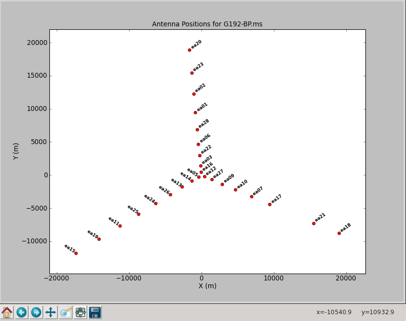
To plot up the antenna positions in the array:
# In CASA
plotants('G192_6s.ms')
NOTE: if after this point (or any other) you get "table locks", which may occur erroneously and are sometimes triggered by plotting tasks, use clearstat to clear them:
# In CASA
clearstat
Now we examine the MS looking for bad data to flag. We will use plotms to bring up an interactive GUI that will display 2-D Y vs. X style line plots. As of CASA 4.4 some of the tabs on the left have changed compared to earlier versions. "Iter" has been changed to "Page" as more options became available. And we introduced "Calibration" to upload a cal-library file.
NOTE: We do not recommend using the editing/flagging features of plotms. It is very easy to mess up your data this way. Also, to improve speed we will be restricting the scope of plotting, so most box/flag operations would not get rid of all the bad data -- although they would appear to delete it, which is misleading.
We will instead use plotms to identify bad data and then use flagcmd to flag it. This will also allow full scripting of the flagging, which is ultimately the best way to keep track of what's been deleted. Given the large dataset sizes now being generated, reproducibility is extremely important. Imagine spending a day flagging your data, then a disk error corrupts the MS: it's imperative that you have an automated way to regenerate your work! This is also why we also encourage you to keep a running file with all the commands you use to process a dataset.
NOTE: If you need an introduction to plotms, see:
- Data flagging with plotms
- Averaging data in plotms
- What's the difference between Antenna1 and Antenna2? Axis definitions in plotms
WARNING: The Flag ![]() button on the plotms GUI is close to other buttons you will be using, in particular the one that deletes boxes you have drawn
button on the plotms GUI is close to other buttons you will be using, in particular the one that deletes boxes you have drawn ![]() . Be careful you don't hit the Flag button by mistake!
. Be careful you don't hit the Flag button by mistake!
To get an idea of the data layout, plot a single baseline (ea02&ea05), channel (31, for all spectral windows), and polarization (RR) versus time. Note that limiting the selected data with appropriate filters is extremely helpful when plotting large datasets:
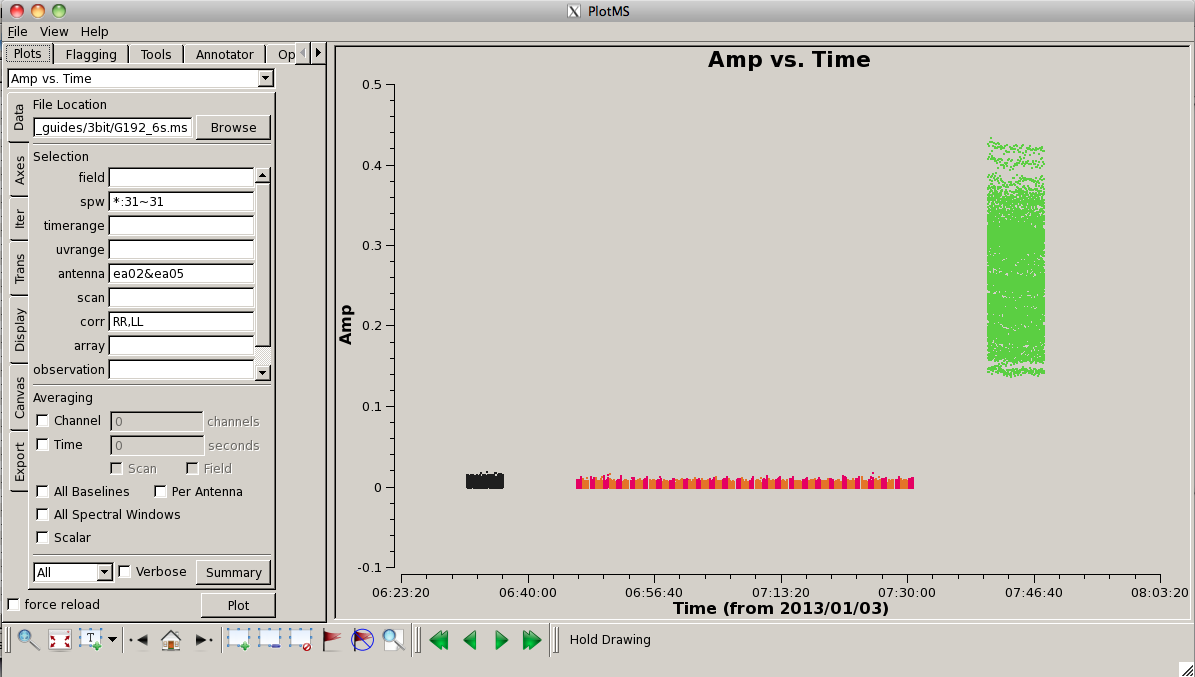
# In CASA
plotms(vis='G192_6s.ms', field='', spw='*:31~31', \
       antenna='ea02&ea05', xaxis='time', yaxis='amp', \
       correlation='rr', coloraxis='field')
Here, we can see the alternating phase calibration and science target scans, as well as the (brighter) bandpass calibrator at the end of the observation. Feel free to play with ways to view. For example, you can change the size of the plotted points, if they are too small to see easily, by setting "Unflagged Points Symbol" to "Custom" and increasing the number of pixels under "Style." You can also experiment with data averaging, plotting different correlations (if you're not doing polarization calibration, you can ignore the "cross-hand" correlations RL and LR and focus on "parallel-hand" correlations RR and LL), changing the plotted axes, altering the colorization scheme (try colorizing by baseline, correlation, field, etc.).
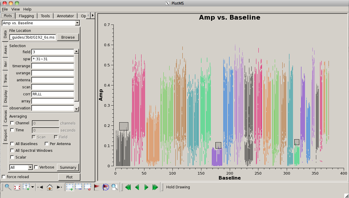
Look for bad antennas by picking the bandpass calibrator and plotting baselines. We color the points by "antenna1" to see which antennas might be troublesome:
# In CASA
plotms(vis='G192_6s.ms', field='3', spw='*:31~31', \
       antenna='', xaxis='baseline',\
       yaxis='amp', coloraxis='antenna1')
You should be able to see that three of the antennas have lower amplitudes than the rest. Boxing with the Mark Regions ![]() tool and using the Locate
tool and using the Locate ![]() tool will show in the logger that these are antennas ea01, ea10 and ea19; indeed, checking the Operator Log for this observation shows that these antennas have collimation offsets and that the data have been corrupted. We will delete these antennas.
tool will show in the logger that these are antennas ea01, ea10 and ea19; indeed, checking the Operator Log for this observation shows that these antennas have collimation offsets and that the data have been corrupted. We will delete these antennas.
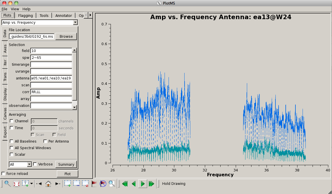
Now look at the raw spectral bandpasses of baselines to ea05. It is in the inner core of the array and a prospective reference antenna. Since we plan to flag them, we will exclude antennas ea01, ea10, and ea19 using negation (represented by "!") in the selection, and iterate by antenna:
# In CASA
plotms(vis='G192_6s.ms', field='3', \
       antenna='ea05;!ea01;!ea10;!ea19', \
       xaxis='frequency', yaxis='amp', \
       coloraxis='corr', iteraxis='antenna')
As you iterate through baselines with ea05, you'll notice that the plot for ea05&ea13 shows that ea13's RCP (correlation = "RR") is weak, as noted in the log file as well. We will flag this antenna over all correlations, since current restrictions do not allow for single-polarization data to be imaged if it's part of a full-polarization dataset.
Also, note that spectral windows 16 through 31 (the upper baseband) for antenna ea18 look very suspicious. We need to keep an eye on these data.
For antenna ea24, there appear to be some issues with spectral windows 47 and 48, and the RCP of spw 40 also looks problematic, so we'll flag this as well.
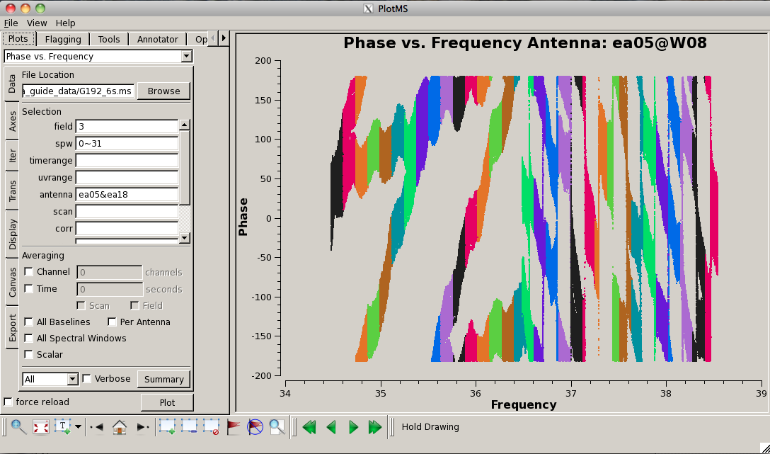
Now plot the phases, iterating through baselines to ea05:
# In CASA
plotms(vis='G192_6s.ms', field='3', \
       antenna='ea05;!ea01;!ea10;!ea13;!ea19', \
       xaxis='frequency', yaxis='phase', \
       coloraxis='spw', iteraxis='antenna')
Notice the rapidly winding phases with frequency due to residual instrumental delays (we will calibrate the instrumental delays and smooth-out the phases later). Most span a turn or less over each 128-MHz subband, but there are some outliers. Step through to ea18. You will see that there are large jumps between spectral windows for spw 16-31 (see plot on the right). This reinforces our suspicion that something is wrong with these data on ea18 and we will flag them as well.
To carry out the flagging, we again use flagcmd in the mode where it takes a list of command strings:
# In CASA: bandpass calibrator analysis flagging
flaglist = ['antenna="ea01,ea10,ea19,ea13"',
            'antenna="ea24" spw="40,47~48"',
            'antenna="ea18" spw="16~31"']
flagcmd(vis='G192_6s.ms', inpmode='list', inpfile=flaglist, \
        action='apply', flagbackup=True)
These commands will carry out the flags and add a record of them to the FLAG_CMD table (where they will be marked as applied). Before applying the flags, a backup version of the flags will be stored as flagcmd_1, in case you would like to restore the MS to the state it was in prior to your new flags (this can be done using flagmanager with mode = "restore" and, in this case, versionname = "flagcmd_1").
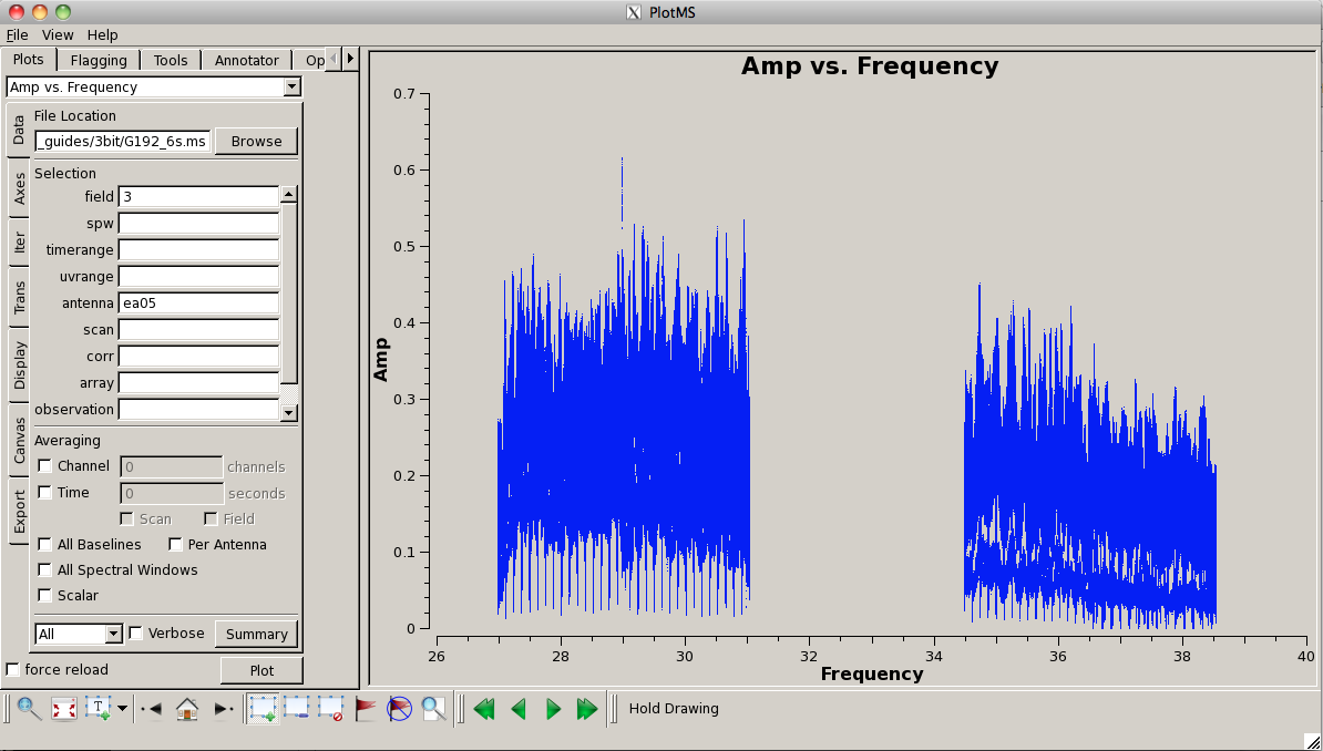
Plot the data again, now that is has been flagged (this time, we'll look at amplitude vs. frequency):
# In CASA
plotms(vis='G192_6s.ms', field='3', antenna='ea05', \
       xaxis='frequency', yaxis='amp')
Now let's look at our phase calibrator -- it is weaker, and we can see some RFI:
# In CASA
plotms(vis='G192_6s.ms', field='1', antenna='ea05', coloraxis = 'spw',\
       correlation = 'RR,LL', xaxis='frequency', yaxis='amp', scan='10,20,30,40,50,60')
Note that we've chosen a subset of scans to limit the amount of data being plotted. This will give us a sense of whether there is serious RFI (or other issues) present in the data, but will obviously not display everything. Later on, when we plot the calibrated data, we will need to again inspect for possible bad data (and we will flag and recalibrate).
Use the Zoom button ![]() , Mark Regions
, Mark Regions ![]() , and Locate
, and Locate ![]() to identify the frequency/channels of the RFI. In particular, we note the following:
to identify the frequency/channels of the RFI. In particular, we note the following:
- 27.228 GHz (spw 33 ch 124)
- 27.707 GHz (spw 37 ch 91)
- 27.81-27.811 GHz (spw 38 ch 66-67)
- 27.819-27.821 GHz (spw 38 ch 75-77)
- 28.894 GHz (spw 46 ch 126)
- 28.976 GHz (spw 48 ch 0)
- 29.684-20.685 GHz (spw 53 ch 68-69)
- 30.976 GHz (spw 63 ch 80) very strong
- 35.782 GHz (spw 10 ch 26)
- 36.523 GHz (spw 15 ch 127)
- 37.946 GHz (spw 27 ch 62)
- 37.948 GHz (spw 27 ch 64)
Flag these channels:
# In CASA: RFI phase calibrator flagging
flaglist = ['spw="33:124,37:91,38:66~67;75~77,46:126,48:0"', \
            'spw="53:68~69,63:80,10:26,15:127,27:62,27:64"']
flagcmd(vis='G192_6s.ms', inpmode='list', inpfile=flaglist, \
        action='apply', flagbackup=True)
When this is finished, it's useful to have a look at the flagged data. To reload the plotms window after taking the new flags into account, check the "force reload" box on the lower left of the plotms GUI and click on "Plot." (As a shortcut, you can also hold down the "Shift" key while clicking on the "Plot" button to force-reload a plot.)
Finally, split off the good data, without retaining the flagged data. This will allow us to work on the data without having to start completely over (if we mess something up badly), as well as let us do simpler data selections (since the data size will be a bit smaller).
# In CASA: splitting good and bad data
# Remove any existing split data, otherwise split will not happen
rmtables('G192_flagged_6s.ms')
split(vis='G192_6s.ms', outputvis='G192_flagged_6s.ms', \
      datacolumn='data', keepflags=False)
- keepflags=False: again, to limit the size of the MS, we do not propagate flagged data to the split-off MS.
You now have a MS called G192_flagged_6s.ms in your working area. This should be 16GB in size, which you can determine at the CASA command prompt by typing:
# In CASA
os.system('du -sh G192_flagged_6s.ms')
Note that the built-in system function allows one to execute UNIX shell commands within a CASA session. (Some, like ls, don't need this extra wrapper, but most are not automatically understood.)
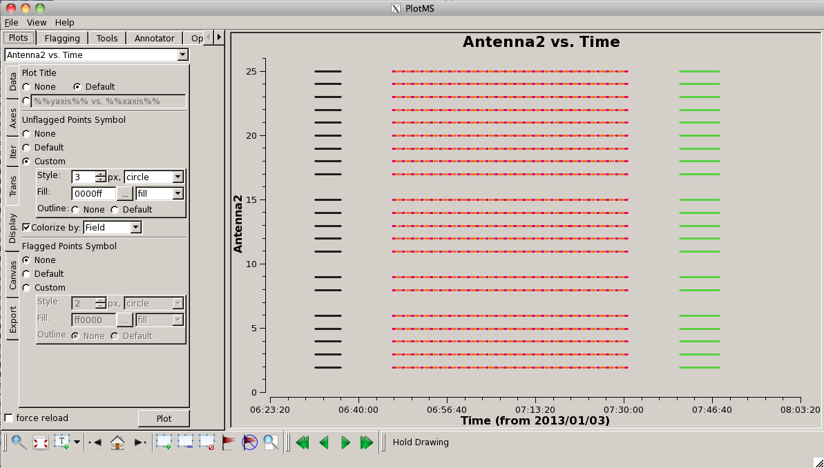
At this point it is useful to plot a "datastream" view of the MS to show which antennas are present at different times. You can do this using:
# In CASA
plotms(vis='G192_flagged_6s.ms', xaxis='time', yaxis='antenna2', \
       symbolshape = 'circle', plotrange=[-1,-1,0,26], coloraxis='field')
This shows the times where data is present on baselines to a given antenna (controlled by setting yaxis="Antenna2"). Note that this means there is no "line" plotted for ea01 (antenna 0). You can pick-up ea01 (and drop ea28) by setting yaxis='antenna1'. To the right we show this plot. You can see that, for the most part, all antennas are present for the entire observation. One exception to this is antenna ea16, which comes in a little late on the first scan of G192.
Calibration
Before proceeding with calibration, we will summarize the split flagged MS:
# In CASA: split and flagged listobs
listobs('G192_flagged_6s.ms', listfile='G192_flagged_listobs.txt')
As before, inspection of the listobs output text file shows that there are now 6,958,621 data records present, and 22 antennas remaining in the MS.
Setting the flux density scale
It is now time to begin calibration! The general data reduction strategy is to derive a series of scaling factors or corrections from the calibrators, which, in addition to a priori calibration information, are collectively applied to the science target. For much more discussion of the philosophy, strategy, and implementation of calibration of synthesis data within CASA, see Synthesis Calibration in the CASA Cookbook and User Reference Manual .
The first step is to insert a model for our flux calibrator source (3C147) into the MS in order to set the flux density scale for bootstrapping to other sources. In order to do this, we first have to locate the model image on our system with setjy. The setjy task has an option to list available model images:
# In CASA
setjy(vis='G192_flagged_6s.ms', listmodels=True)
which sends output to your terminal (but not the logger). For example, on an NRAO workstation, we obtain the following:
No candidate modimages matching '*.im* *.mod*' found in .

Candidate modimages (*) in /home/casa/packages/RHEL6/release/casa-release-XXX/data/nrao/VLA/CalModels:
3C138_A.im  3C138_Q.im	3C147_A.im  3C147_Q.im	3C286_A.im  3C286_Q.im	3C48_A.im  3C48_Q.im  README
3C138_C.im  3C138_S.im	3C147_C.im  3C147_S.im	3C286_C.im  3C286_S.im	3C48_C.im  3C48_S.im
3C138_K.im  3C138_U.im	3C147_K.im  3C147_U.im	3C286_K.im  3C286_U.im	3C48_K.im  3C48_U.im
3C138_L.im  3C138_X.im	3C147_L.im  3C147_X.im	3C286_L.im  3C286_X.im	3C48_L.im  3C48_X.im

No candidate modimages matching '*.im* *.mod*' found in .
The relevant image for our purposes is 3C147_A.im, in the subdirectory //data/nrao/VLA/CalModels/. Your system may show a different location (for example /home/casa/data/nrao/VLA/CalModels/ of your CASA installation. Since CASA knows about this image, we only have to give the image name and not the entire path. Note that outside of the NRAO, you may need to provide setjy with the entire path along with the model image name (this depends on your platform and installation location).
We can now run the setjy task using the appropriate model:
# In CASA: model for the flux calibrator
setjy(vis='G192_flagged_6s.ms', field='0', scalebychan=True, \
      standard='Perley-Butler 2010', model='3C147_A.im')
- scalebychan=True: will fill the model with per-channel values; otherwise, setjy would use a single value per spectral window.
- usescratch=False: put the model in the header instead of creating scratch columns in the MS. This will take up considerably less disk space.
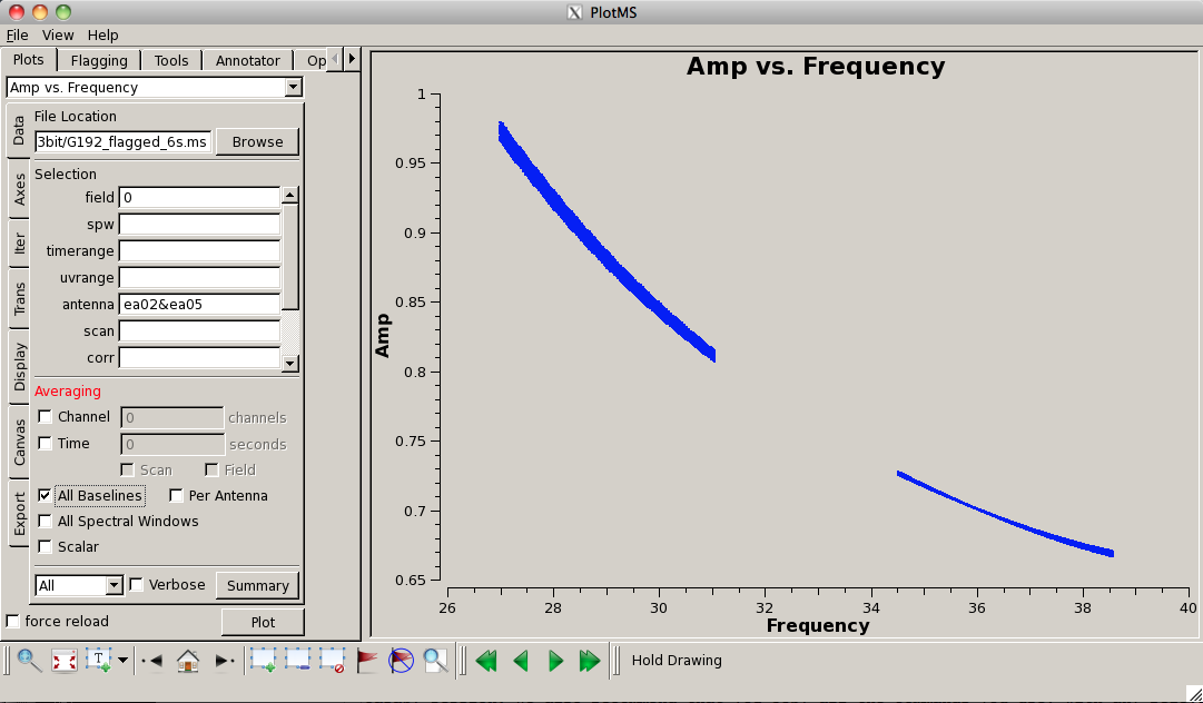
We can plot the model data using plotms:
# In CASA
plotms(vis='G192_flagged_6s.ms', field='0', antenna='ea02&ea05', \
       xaxis='freq', yaxis='amp', ydatacolumn='model')
Inspecting the logger report shows that 3C147 has a flux density of 1.4061 Jy at the lower end of the band (spw 63; ~31 GHz) and 1.2779 Jy at the upper end (spw 0; ~35 GHz).
Deriving a priori calibrations
Some calibration products are carried along throughout the calibration process and used as priors for subsequent calibration steps. These include the antenna position corrections, gain-elevation curves, tropospheric opacity corrections, and requantizer gains.
Antenna position corrections
We use gencal to determine any antenna-position corrections that need to be applied to the data. This is based on a database of corrections with the dates and times the corrections were determined and when they were included in the online observing system.
# In CASA: determining antenna position corrections
gencal('G192_flagged_6s.ms', caltable='calG192.antpos', \
       caltype='antpos', antenna='')
You should see in the logger:
Determine antenna position offests from the baseline correction database
gencal	offsets for antenna ea05 : -0.00100   0.00000   0.00290
gencal	offsets for antenna ea16 : -0.00310   0.00000   0.00100
So this dataset does require antenna position corrections on ea05 & ea16. If no corrections were necessary, the output from gencal would have appeared as follows:
No offsets found for this MS
*** Warning *** No offsets found. No caltable created.
gencal::::casa	An error occurred running task gencal.
Although the "warning" makes it seem as if the task has failed, the message is normal and means there simply aren't any antenna corrections to apply.
Gain-elevation curves
We will use gencal to create calibration tables containing the gain curves and tropospheric opacity corrections for the antennas. Note that the gaincurve=True option that was previously available in calibration tasks (e.g., bandpass) is no longer available as of CASA 4.2. The syntax for generating a gaincurve calibration table in gencal is as follows:
# In CASA: generating gaincurve calibration
gencal('G192_flagged_6s.ms', caltable='calG192.gaincurve', \
       caltype='gc')
Tropospheric opacity corrections

The atmospheric opacity during the observations can be computed from a seasonal model and/or weather station information. We will use the plotweather task to display the weather information and to calculate the zenith opacities for each spectral window. After the zenith opacities are derived, gencal will recompute the correct elevation of the data automatically using [math]\displaystyle{ e^{(-\csc[el]\tau_z)} }[/math] and create the opacity-correction calibration table.
To start, we want to plot the opacity of the atmosphere at the time these observations was taken. plotweather plots the weather conditions during the observations and calculates the atmospheric opacities based on these data, in combination with a seasonal model that contains long-term statistics at the VLA site. Using seasonal_weight=0.5 (the default value) gives equal weights to the seasonal model and weather station data:
We will be running plotweather in a way that will assign the opacity list (one entry for each spectral window in ascending order) to the variable myTau:
# In CASA
myTau = plotweather(vis='G192_flagged_6s.ms', doPlot=T)
The logger should display:
##########################################
##### Begin Task: plotweather        #####
plotweather(vis="G192_flagged_6s.ms",seasonal_weight=0.5,doPlot=True,plotName="")
2013-06-18 21:47:00 INFO plotweather	SPW : Frequency (GHz) : Zenith opacity (nepers)
 0  :   34.476  :  0.03
 1  :   34.604  :  0.031
 2  :   34.732  :  0.031
 3  :   34.860  :  0.031
 4  :   34.988  :  0.032
<snip>
61  :   30.640  :  0.024
62  :   30.768  :  0.024
63  :   30.896  :  0.024
wrote weather figure: G192_flagged_6s.ms.plotweather.png
##### End Task: plotweather          #####
##########################################
In addition to assigning the myTau variable to the full list of opacities per spw, plotweather also creates a file G192_flagged_6s.ms.plotweather.png with the elevation of the sun, the wind speed and direction, the temperature, and precipitable water vapor (PWV) as functions of time over the course of the observation (view this file with your preferred image viewer like gthumb, xv, or Preview).
We can now create a calibration table to correct for the atmospheric opacity with gencal using the calmode='opac' parameter. We could input the opacities directly, but it's easier to use the myTau variable defined above:
# In CASA: generate atmospheric opacity calibration
gencal(vis='G192_flagged_6s.ms', caltable='calG192.opacity', \
       caltype='opac', spw='0~63', parameter=myTau)
Requantizer gain corrections
Finally, we will use gencal to create a calibration table containing corrections for the requantizer gains. Although this is only necessary for 3-bit data, such as our G192 dataset, it can be done for 8-bit datasets without any ill effects. For 3-bit data, this step is needed to account for the small gain changes (~5-10%) that result from resetting the quantizer gains as the correlator changes to a new 3-bit configuration. (Here is more information on observing with the 3-bit system.)
# In CASA: generate requantizer gains corrections
gencal('G192_flagged_6s.ms', caltable='calG192.requantizer', \
       caltype='rq')
The caltables we have generated (calG192.antpos, calG192.gaincurve, calG192.opacity, and calG192.requantizer) will need to be pre-applied in subsequent calibration steps.
Calibrating delays and initial bandpass solutions
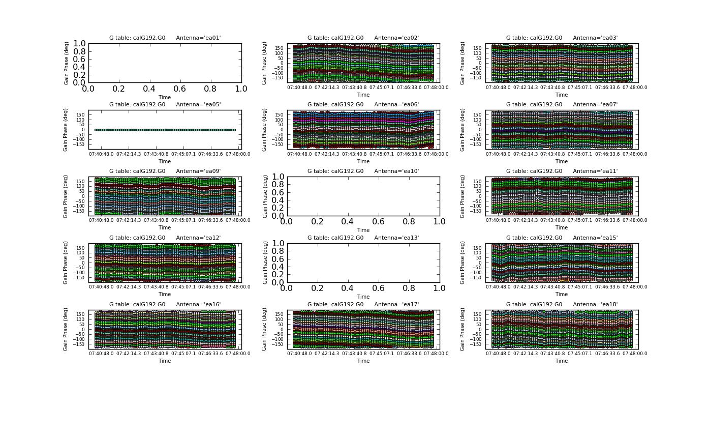
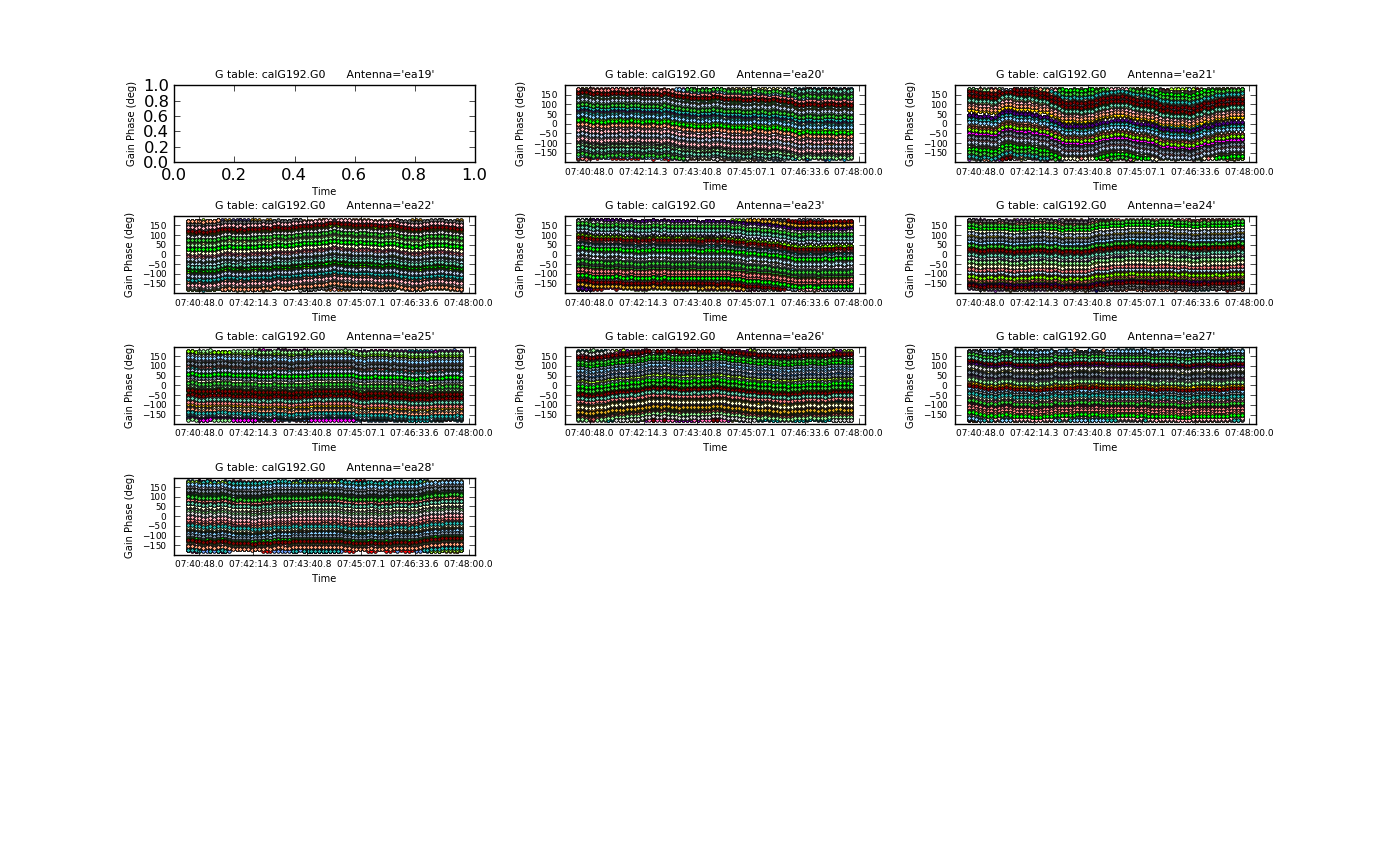
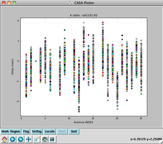


First, we do a phase-only calibration solution on a narrow range of channels near the center of each spectral window on the bandpass calibrator 3C84 to flatten them with respect to time before solving for the bandpass. The range 60~68 should work. Pick a reference antenna near the center of the array -- ea05 is a reasonable choice (see above):
# In CASA: phase only calibration
gaincal(vis='G192_flagged_6s.ms', caltable='calG192.G0', \
        field='3', spw='*:60~68', \
        gaintable=['calG192.antpos','calG192.gaincurve', \
                   'calG192.requantizer','calG192.opacity'], \
        gaintype='G', refant='ea05', calmode='p', \
        solint='int', minsnr=3)
- refant='ea05' : Use ea05 as the reference antenna
- solint='int' : Do a per-integration solve (every 6 seconds, since we've time-averaged the data).
- minsnr=3 : Apply a minimum signal-to-noise cutoff. Solutions with less than this value will be flagged.
- gaintable=['calG192.antpos', 'calG192.gaincurve', 'calG192.requantizer', 'calG192.opacity'] : Pre-apply the antenna position corrections, gaincurve, opacity, and requantizer calibration tables.
Plot the phase solutions (using full phase range, -180 to 180, instead of autorange):
# In CASA
plotcal(caltable='calG192.G0', xaxis='time', yaxis='phase', \
        iteration='antenna', plotrange=[-1,-1,-180,180])
Step through the antenna-based solutions. They look good (and fairly flat over the scans).
NOTE: When you are done plotting and want to use the calibration table in another task (e.g., for subsequent calibration or viewing with plotms), use the Quit button on the GUI to dismiss the plotter and free-up the lock on the calibration table. You should see a message in your terminal window saying "Resetting plotcal" which means you are good to go!
If you want to make single-page, multipanel plots (like those shown to the right), particularly for a hardcopy (where it only shows the first page), you can do:
# In CASA
plotcal(caltable='calG192.G0', xaxis='time', yaxis='phase', \
        antenna='0~10,12~15', subplot=531, iteration='antenna', \
        plotrange=[-1,-1,-180,180], fontsize=8.0, \
        markersize=3.0, figfile='plotG192_plotcal_G0p1.png')
plotcal(caltable='calG192.G0', xaxis='time', yaxis='phase', \
        antenna='16~26', subplot=531, iteration='antenna', \
        plotrange=[-1,-1,-180,180], fontsize=8.0, \
        markersize=3.0, figfile='plotG192_plotcal_G0p2.png')
We can now solve for the residual delays that we saw in plotms when we plotted phase vs. frequency. This uses the gaintype='K' option in gaincal. Note that this currently does not do a "global fringe-fitting" solution for delays, but instead does a baseline-based delay solution for all baselines to the reference antenna, treating these as antenna-based delays. In most cases with high-enough S/N to get baseline-based delay solutions, this will suffice. We avoid the edge channels of each spectral window by selecting channels 5~122:
# In CASA: residual delays
gaincal(vis='G192_flagged_6s.ms', caltable='calG192.K0', \
        gaintable=['calG192.antpos', 'calG192.gaincurve', 'calG192.requantizer', \
                   'calG192.opacity', 'calG192.G0'], \
        field='3', spw='*:5~122', gaintype='K', \
        refant='ea05', solint='inf', minsnr=3)
Note that we have also pre-applied our initial phase table, calG192.G0. We can plot the delays, in nanoseconds, as a function of antenna index (you will get one for each spw and polarization):
# In CASA
plotcal(caltable='calG192.K0', xaxis='antenna', yaxis='delay')
The delays range from around -5 to 4 nanoseconds.
Now we solve for the antenna bandpasses using the previous tables:
# In CASA: antenna bandpasses
bandpass(vis='G192_flagged_6s.ms', caltable='calG192.B0', \
         gaintable=['calG192.antpos', 'calG192.gaincurve', 'calG192.requantizer', \
                    'calG192.opacity', 'calG192.G0', 'calG192.K0'], \
         field='3', refant='ea05', solnorm=False, \
         bandtype='B', solint='inf')
WARNING: You must set solnorm=False here or later on you will find some offsets among spws due to the way the amplitude scaling adjusts weights internally during solving.

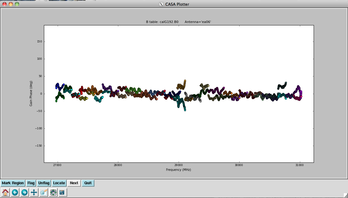
You will see in the terminal some reports of solutions failing due to "Insufficient unflagged antennas" -- note that these are for the channels we flagged earlier.
This is the first amplitude-scaling calibration that we do, so it is important to have used the calG192.gaincurve caltable (or set gaincurve=True) as well as the calG192.opacity caltable (or set opacity appropriately).
Plot the resulting bandpasses in amplitude and phase:
# In CASA
plotcal(caltable='calG192.B0', xaxis='freq', yaxis='amp', \
        spw='0~31', iteration='antenna')
#
plotcal(caltable='calG192.B0', xaxis='freq', yaxis='amp', \
        spw='32~63', iteration='antenna')
#
plotcal(caltable='calG192.B0', xaxis='freq', yaxis='phase', \
        iteration='antenna', spw='0~31', \
        plotrange=[-1,-1,-180,180])
#
plotcal(caltable='calG192.B0', xaxis='freq', yaxis='phase', \
        iteration='antenna', spw='32~63', \
        plotrange=[-1,-1,-180,180])
In the bandpass phases you no longer see the residual antenna delays (just residual spw phase offsets from the delay solution registration), but there are some band edge effects apparent.
Bootstrapping the bandpass calibrator spectrum
Unfortunately, our flux density calibrator was not bright enough at Ka-band to use as the bandpass calibration source. Since there is no a priori spectral information for our chosen bandpass calibrator, 3C84, we need to bootstrap to find its spectral index, then recalibrate with this information in order to avoid folding the intrinsic spectral shape of 3C84 into our calibration.
First, we use the initial round of bandpass calibration to create gain solutions for the flux and bandpass calibrators:
# In CASA: flux and bandpass calibrators gain
gaincal(vis='G192_flagged_6s.ms', caltable='calG192.G1', field='0,3', \
        gaintable=['calG192.antpos', 'calG192.gaincurve', 'calG192.requantizer', \
                   'calG192.opacity', 'calG192.K0', \
                   'calG192.B0'], \
        gaintype='G', refant='ea05', calmode='ap', solint='30s', minsnr=3)
Now let's have a look at the phase and amplitude solutions, iterating over antenna. We will look at the flux calibrator (3C147) and bandpass calibrator (3C84) individually since they're widely separated in time:
# In CASA
plotcal(caltable='calG192.G1', xaxis='time', yaxis='amp', \
        field='0', iteration='antenna')
#
plotcal(caltable='calG192.G1', xaxis='time', yaxis='amp', \
        field='3', iteration='antenna')
#
plotcal(caltable='calG192.G1', xaxis='time', yaxis='phase', \
        iteration='antenna', plotrange=[-1,-1,-180,180], \
        field='0')
#
plotcal(caltable='calG192.G1', xaxis='time', yaxis='phase', \
        iteration='antenna', plotrange=[-1,-1,-180,180], \
        field='3')
The solutions all look reasonable and relatively constant with time.
Now that we have gain solutions for the flux and bandpass calibrators, we can use fluxscale to scale the gain amplitudes of the bandpass calibrator:
# In CASA: bandpass calibrator gain amplitudes scaling
flux1 = fluxscale(vis='G192_flagged_6s.ms', caltable='calG192.G1', \
                  fluxtable='calG192.F1', reference='0', \
                  transfer='3', listfile='3C84.fluxinfo', fitorder=1)
- flux1 = fluxscale(...): by providing a variable flux1, we allow fluxscale to use this for the output Python dictionary it returns with lots of information about the flux scaling. You can inspect the output dictionary flux1 by typing "print flux1" at the CASA command line.
- fluxtable='calG192.F1': this is the output scaled gain table. Since we are only using this to find the spectral index of 3C84, we won't be using this table.
- listfile='3C84.fluxinfo': an output file that contains the derived flux values and fit information.
- fitorder=1: only find a spectral index, ignoring curvature in the spectrum.
The last line in the file (and displayed in the logger) shows:
Fitted spectrum for 3c84-J0319+413 with fitorder=1: Flux density = 31.454 +/- 0.0310638 (freq=32.5128 GHz) spidx=-0.493668 +/- 0.00820698

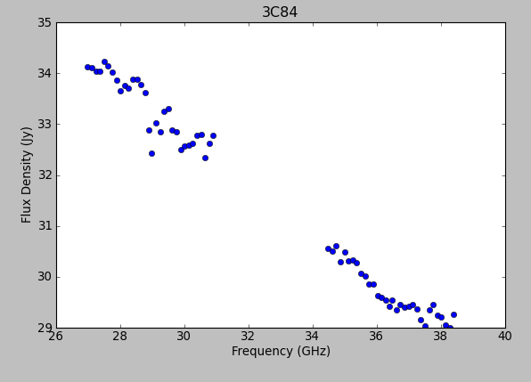
Using the information in the returned flux dictionary, we can plot the derived spectrum:
# In CASA
freq = flux1['freq'] / 1e9
spw_list = range(0,64)
spw_str = []
for i in spw_list:
   thisspw = str(i)
   spw_str.append(thisspw)

bootstrapped_fluxes = []
for j in spw_str:
    thisflux = flux1['3'][j]['fluxd'][0]
    if thisflux ==None:
        continue
    else:
        bootstrapped_fluxes.append(thisflux)

pl.clf()
pl.plot(freq, bootstrapped_fluxes, 'bo')
pl.xlabel('Frequency (GHz)')
pl.ylabel('Flux Density (Jy)')
pl.title('3C84')
pl.show()
Note the bump around 37 GHz -- what is this? We will not be able to account for it with the simple spectral index model, but still, ours is a good first approximation.
We can use the model from fluxscale to fill the MODEL column with 3C84's spectral information using setjy:
# In CASA: spectral information
setjy(vis='G192_flagged_6s.ms', field='3', scalebychan=True, \
      standard = 'manual', fluxdensity=[29.8756, 0, 0, 0], spix=-0.598929, \
      reffreq='32.4488GHz')
Checking with plotms that the data have been appropriately filled:
# In CASA
plotms(vis='G192_flagged_6s.ms', field='3', antenna='ea05&ea02', \
       xaxis='freq', yaxis='amp', ydatacolumn='model')
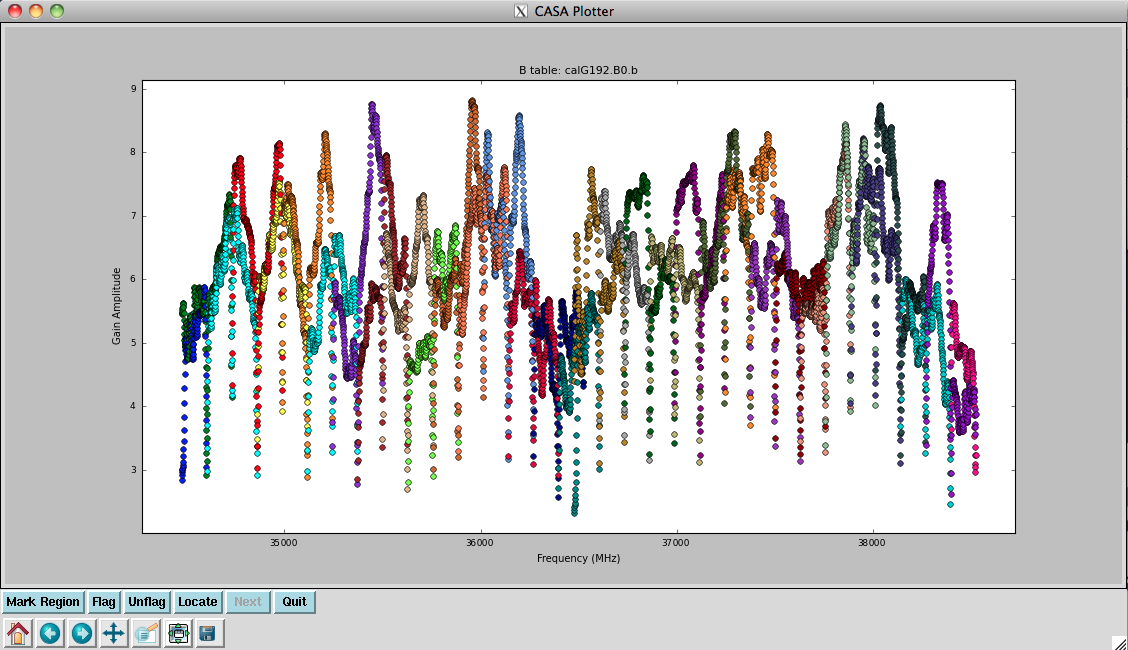

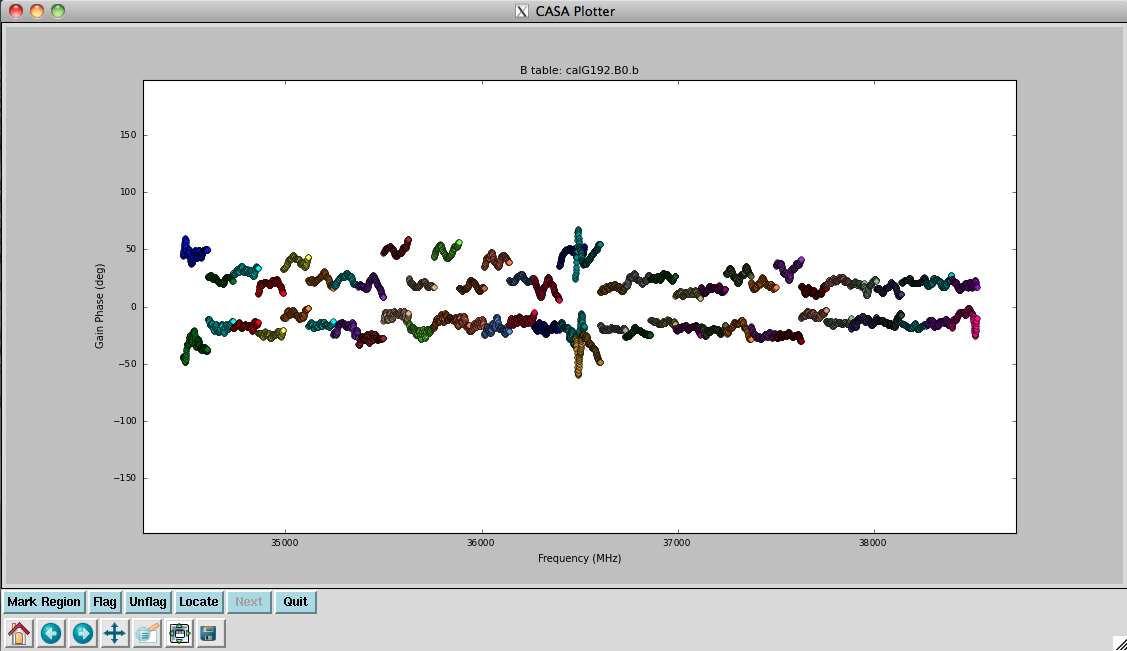
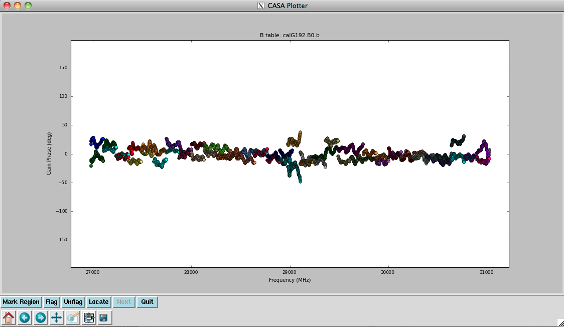
Finally, we redo the previous calibration using this new model information. Although the commands are the same as what we issued earlier, keep in mind that the model values for the bandpass calibrator have changed, and therefore the results of these calibration calculations will differ:
# In CASA: phase only recalibration
gaincal(vis='G192_flagged_6s.ms', caltable='calG192.G0.b', \
        field='3', spw='*:60~68', \
        gaintable=['calG192.antpos', 'calG192.gaincurve', \
                   'calG192.requantizer', 'calG192.opacity'], \
        gaintype='G', refant='ea05', calmode='p', \
        solint='int', minsnr=3)
# In CASA: residual delays recalibration
gaincal(vis='G192_flagged_6s.ms', caltable='calG192.K0.b', \
        gaintable=['calG192.antpos', 'calG192.gaincurve', 'calG192.requantizer', \
                  'calG192.opacity', 'calG192.G0.b'], \
        field='3', spw='*:5~122', gaintype='K', \
        refant='ea05', solint='inf', minsnr=3)
# In CASA: antenna bandpasses recalibration
bandpass(vis='G192_flagged_6s.ms', caltable='calG192.B0.b', \
         gaintable=['calG192.antpos', 'calG192.gaincurve', 'calG192.requantizer', \
                    'calG192.opacity', 'calG192.G0.b', 'calG192.K0.b'], \
         field='3', refant='ea05', solnorm=False, \
         bandtype='B', solint='inf')
It's a good idea to inspect these solutions as well:
# In CASA
plotcal(caltable='calG192.B0.b', xaxis='freq', yaxis='amp', \
        spw='0~31', iteration='antenna')
#
plotcal(caltable='calG192.B0.b', xaxis='freq', yaxis='amp', \
        spw='32~63', iteration='antenna')
#
plotcal(caltable='calG192.B0.b', xaxis='freq', yaxis='phase', \
        iteration='antenna', spw='0~31', \
        plotrange=[-1,-1,-180,180])
#
plotcal(caltable='calG192.B0.b', xaxis='freq', yaxis='phase', \
        iteration='antenna', spw='32~63', \
        plotrange=[-1,-1,-180,180])
They look virtually unchanged from the previous solutions, with the exception that the amplitude scaling is corrected for the spectrum of 3C84. Now that we have the final version of our bandpass calibration, we can proceed to the full calibration of the dataset.
Final phase and amplitude calibration

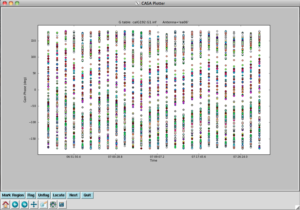
Now we will compute the calibrators' gain phases using the full bandwidth. We will do the calibrators one at a time and append subsequent solutions, since we will use different solution intervals. For 3C147 and 3C84, we obtain one solution per integration (these are bright enough); for the phase calibrator, J0603+174, we will use 12 second solution intervals:
# In CASA: compute gain phases using 3C147
gaincal(vis='G192_flagged_6s.ms', caltable='calG192.G1.int', \
        gaintable=['calG192.antpos', 'calG192.gaincurve', 'calG192.requantizer', \
                   'calG192.opacity', 'calG192.K0.b', 'calG192.B0.b'], \
        field='0', refant='ea05', solnorm=F, \
        solint='int', gaintype='G', calmode='p')
# In CASA: compute gain phases using J0603+174
gaincal(vis='G192_flagged_6s.ms', caltable='calG192.G1.int', \
        gaintable=['calG192.antpos', 'calG192.gaincurve', 'calG192.requantizer', \
                   'calG192.opacity', 'calG192.K0.b', 'calG192.B0.b'], \
        field='1', refant='ea05', solnorm=F, \
        solint='12s', gaintype='G', calmode='p', append=True)
# In CASA: compute gain phases using 3C84
gaincal(vis='G192_flagged_6s.ms', caltable='calG192.G1.int', \
        gaintable=['calG192.antpos', 'calG192.gaincurve', 'calG192.requantizer', \
                   'calG192.opacity', 'calG192.K0.b', 'calG192.B0.b'], \
        field='3', refant='ea05', solnorm=F, \
        solint='int', gaintype='G', calmode='p', append=True)
These will get applied when solving for amplitudes (see the "G2" calibration tables below), and when calibrating the calibrators themselves (with the task applycal).
The phases track nicely with time:
# In CASA
plotcal(caltable='calG192.G1.int', xaxis='time', yaxis='phase', \
        iteration='antenna', plotrange=[-1,-1,-180,180])
To apply phase calibration to the target, we will make a second table for the gain calibrator (J0603+174) with one solution per scan:
# In CASA: applying phase calibration
gaincal(vis='G192_flagged_6s.ms', caltable='calG192.G1.inf', \
        gaintable=['calG192.antpos', 'calG192.gaincurve', 'calG192.requantizer', \
                   'calG192.opacity', 'calG192.K0.b', 'calG192.B0.b'], \
        field='1', refant='ea05', solnorm=F, \
        solint='inf', gaintype='G', calmode='p')
These phase gain solutions in calG192.G1.inf will be interpolated by applycal onto our target. These look good as well:
# In CASA
plotcal(caltable='calG192.G1.inf', xaxis='time', yaxis='phase', \
        iteration='antenna', plotrange=[-1,-1,-180,180])
Now, let's solve for amplitudes on a per-scan interval, after applying the per-integration phases. Do these separately using gainfield so phases don't get transferred across fields. Note that gaincal uses linear interpolation of the previously determined phases by default. This is generally fine; we will set the interpolation to "nearest" (in time).
# In CASA: 3C147 scan solving amplitudes
gaincal(vis='G192_flagged_6s.ms', caltable='calG192.G2', \
        gaintable=['calG192.antpos', 'calG192.gaincurve', 'calG192.requantizer', \
                   'calG192.opacity', 'calG192.K0.b', 'calG192.B0.b', 'calG192.G1.int'], \
        gainfield=['', '', '', '', '3', '3', '0'], \
        interp=['', '', '', '', 'nearest', 'nearest', 'nearest'], \
        field='0', refant='ea05', solnorm=F, \
        solint='inf', gaintype='G', calmode='a')

# In CASA: J0603+174  scan solving amplitudes
gaincal(vis='G192_flagged_6s.ms', caltable='calG192.G2', \
        gaintable=['calG192.antpos', 'calG192.gaincurve', 'calG192.requantizer', \
                   'calG192.opacity', 'calG192.K0.b', 'calG192.B0.b', 'calG192.G1.int'], \
        gainfield=['', '', '', '', '3', '3', '1'], \
        interp=['', '', '', '', 'nearest', 'nearest', 'nearest'], \
        field='1', refant='ea05', solnorm=F, \
        solint='inf', gaintype='G', calmode='a', append=True)
# In CASA: 3C84 scan solving amplitudes
gaincal(vis='G192_flagged_6s.ms', caltable='calG192.G2', \
        gaintable=['calG192.antpos', 'calG192.gaincurve', 'calG192.requantizer', \
                   'calG192.opacity', 'calG192.K0.b', 'calG192.B0.b', 'calG192.G1.int'], \
        gainfield=['', '', '', '', '3', '3', '3'], \
        interp=['', '', '', '', 'nearest', 'nearest', 'nearest'], \
        field='3', refant='ea05', solnorm=F, \
        solint='inf', gaintype='G', calmode='a', append=True)
#
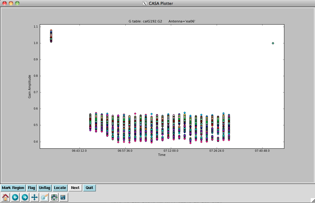
Let's have a look at the amplitudes:
# In CASA
plotcal(caltable='calG192.G2', xaxis='time', yaxis='amp', \
        iteration='antenna')
We will apply this table (calG192.G2) to the data.
First, we need to use fluxscale to transfer the amplitude solutions from 3C147:
# In CASA: using fluxscale to transfer the amplitude solutions
flux2 = fluxscale(vis='G192_flagged_6s.ms', caltable='calG192.G2', \
                  fluxtable='calG192.F2', reference='0')
where we have now captured the return dictionary in the Python object flux2.
The logger output gives:
Found reference field(s): 3C147
Found transfer field(s):  gcal-J0603+174 3c84-J0319+413
Flux density for gcal-J0603+174 in SpW=0 (freq=3.4476e+10 Hz) is: 0.272996 +/- 0.0107803 (SNR = 25.3236, N = 44)
Flux density for gcal-J0603+174 in SpW=1 (freq=3.4604e+10 Hz) is: 0.272149 +/- 0.0107452 (SNR = 25.3274, N = 44)
Flux density for gcal-J0603+174 in SpW=2 (freq=3.4732e+10 Hz) is: 0.270155 +/- 0.0108101 (SNR = 24.9911, N = 44)
Flux density for gcal-J0603+174 in SpW=3 (freq=3.486e+10 Hz) is: 0.26981 +/- 0.0116108 (SNR = 23.2378, N = 44)
Flux density for gcal-J0603+174 in SpW=4 (freq=3.4988e+10 Hz) is: 0.269297 +/- 0.011425 (SNR = 23.5709, N = 44)
Flux density for gcal-J0603+174 in SpW=5 (freq=3.5116e+10 Hz) is: 0.268182 +/- 0.0109841 (SNR = 24.4155, N = 44)
Flux density for gcal-J0603+174 in SpW=6 (freq=3.5244e+10 Hz) is: 0.267146 +/- 0.0110096 (SNR = 24.2649, N = 44)
<snip>
Flux density for gcal-J0603+174 in SpW=60 (freq=3.0512e+10 Hz) is: 0.286719 +/- 0.0127605 (SNR = 22.4692, N = 44)
Flux density for gcal-J0603+174 in SpW=61 (freq=3.064e+10 Hz) is: 0.283124 +/- 0.012677 (SNR = 22.3337, N = 44)
Flux density for gcal-J0603+174 in SpW=62 (freq=3.0768e+10 Hz) is: 0.283599 +/- 0.012742 (SNR = 22.257, N = 44)
Flux density for gcal-J0603+174 in SpW=63 (freq=3.0896e+10 Hz) is: 0.284513 +/- 0.0129893 (SNR = 21.9036, N = 44)
Flux density for 3c84-J0319+413 in SpW=0 (freq=3.4476e+10 Hz) is: 1.05565 +/- 0.0346701 (SNR = 30.4484, N = 44)
Flux density for 3c84-J0319+413 in SpW=1 (freq=3.4604e+10 Hz) is: 1.06356 +/- 0.0356465 (SNR = 29.8363, N = 44)
Flux density for 3c84-J0319+413 in SpW=2 (freq=3.4732e+10 Hz) is: 1.06441 +/- 0.0347335 (SNR = 30.6452, N = 44)
Flux density for 3c84-J0319+413 in SpW=3 (freq=3.486e+10 Hz) is: 1.06012 +/- 0.0356317 (SNR = 29.7521, N = 44)
<snip>
Flux density for 3c84-J0319+413 in SpW=60 (freq=3.0512e+10 Hz) is: 1.05782 +/- 0.0299479 (SNR = 35.3218, N = 44)
Flux density for 3c84-J0319+413 in SpW=61 (freq=3.064e+10 Hz) is: 1.04535 +/- 0.0303227 (SNR = 34.4743, N = 44)
Flux density for 3c84-J0319+413 in SpW=62 (freq=3.0768e+10 Hz) is: 1.06008 +/- 0.0296807 (SNR = 35.7162, N = 44)
Flux density for 3c84-J0319+413 in SpW=63 (freq=3.0896e+10 Hz) is: 1.06627 +/- 0.0302509 (SNR = 35.2476, N = 44)
Fitted spectrum for gcal-J0603+174 with fitorder=1: Flux density = 0.277387 +/- 0.000375653 (freq=32.4488 GHz) spidx=-0.612043 +/- 0.0112223
Fitted spectrum for 3c84-J0319+413 with fitorder=1: Flux density = 1.04871 +/- 0.00117454 (freq=32.4488 GHz) spidx=0.105074 +/- 0.00933686
You may see slightly different numbers on your machine. Note that "N" here is the number of antennas x the number of polarizations used for the calculations. In this case, there are 22 unflagged antennas and 2 polarizations.
Also, note that the flux-scaled amplitudes for 3C84 are all almost exactly 1 Jy. This is not because the actual flux of 3C84 is 1 Jy, of course. Rather, remember that the spectrum and flux information is now included in the bandpass table. When we apply the calibration, in the next section, you will see that 3C84's flux does indeed come out as expected.
Applying the Calibration and Final Editing
Next we apply all our accumulated calibration tables to the flagged MS. We apply these to the calibration fields individually, using the appropriate gainfields and interpolation for each:
- For 3C147 (field 0) we did per-integration phase solutions and a single scan amplitude, so use "linear" and "nearest" interpolation, respectively;
- for the nearby gain calibrator (field 1) we did 12-s phase and per-scan amplitude solutions, for which we will use "linear" and "nearest" interpolation, respectively;
- for G192 (field 2), we will calibrate with field 1, using the per-scan solutions and "linear" interpolation; and finally,
- for the bandpass calibrator 3C84 (field 3), we did per-integration phase solutions and a single scan amplitude, so use "linear" and "nearest" interpolation respectively.
# In CASA: 3C147 accumulated calibration
applycal(vis='G192_flagged_6s.ms', field='0', \
         gaintable=['calG192.antpos', 'calG192.requantizer', 'calG192.gaincurve', \
                    'calG192.opacity', 'calG192.K0.b', 'calG192.B0.b', \
                    'calG192.G1.int', 'calG192.G2'], \
         gainfield=['', '', '', '', '', '', '0', '0'], \
         interp=['', '', '', '', 'nearest', 'nearest', 'linear', 'nearest'], calwt=False)
# In CASA: gain accumulated calibration
applycal(vis='G192_flagged_6s.ms', field='1', \
         gaintable=['calG192.antpos', 'calG192.requantizer', 'calG192.gaincurve', \
                    'calG192.opacity', 'calG192.K0.b', 'calG192.B0.b', \
                    'calG192.G1.int', 'calG192.F2'], \
         gainfield=['', '', '', '', '', '', '1', '1'], \
         interp=['', '', '', '', 'nearest', 'nearest', 'linear', 'nearest'], calwt=False)
# In CASA: G192 accumulated calibration
applycal(vis='G192_flagged_6s.ms', field='2', \
         gaintable=['calG192.antpos', 'calG192.requantizer', 'calG192.gaincurve', \
                    'calG192.opacity', 'calG192.K0.b', 'calG192.B0.b',\
                    'calG192.G1.inf', 'calG192.F2'], \
         gainfield=['', '', '', '', '', '', '1', '1'], \
         interp=['', '', '', '', 'nearest', 'nearest', 'linear', 'linear'], calwt=False)
# In CASA: 3C84 accumulated calibration
applycal(vis='G192_flagged_6s.ms', field='3', \
         gaintable=['calG192.antpos', 'calG192.requantizer', 'calG192.gaincurve', \
                    'calG192.opacity', 'calG192.K0.b', 'calG192.B0.b', \
                    'calG192.G1.int', 'calG192.F2'], \
         gainfield=['', '', '', '', '', '', '3', '3'], \
         interp=['', '', '', '', 'nearest', 'nearest', 'linear', 'nearest'], calwt=False)
Because we used usesratch=False in setjy, the CORRECTED_DATA scratch column will be created the first time you run applycal. This will take a few minutes to write, increasing the size of the MS to 30 GB, and will store the calibrated data in the calibrated data column of the MS.
IMPORTANT NOTES ON THE USE OF YOUR FLUXSCALE (F2) TABLE IN APPLYCAL:

* When we ran fluxscale and generated table calG192.F2 to transfer the amplitude solutions
from our flux calibrator, fluxscale was run with incremental = False by default.  This
means that the flux density scale correction factors derived from the primary flux calibrator
were applied to the gains of the secondary calibrators.  So, the information from calG192.G2
(which contains the amplitude solutions) is already accounted for in calG192.F2 and we will
NOT need to supply calG192.G2 to our list of calibration tables for our secondary
calibrators and science target fields (in this case, fields 1, 2, and 3 -- we do still need
our G2 table for field 0 though!).

* It is also possible to run fluxscale with incremental = True.  In this case, only the
scale correction factors are written out to the fluxtable, and calG192.G2 would need to be
included in the list of gaintables for ALL fields at the applycal stage.
Now we examine the corrected data for 3C147. We will avoid spectral window edges and bin the data in time and frequency:
# In CASA
plotms(vis='G192_flagged_6s.ms', field='0', \
       xaxis='frequency', yaxis='amp', \
       ydatacolumn='corrected', spw='*:5~122', \
       averagedata=True, avgchannel='8', \
       avgtime='1000s', coloraxis='baseline')
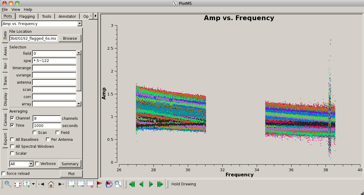
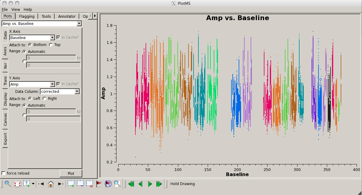
In this plot (see figure above) there is some suspicious data in the frequency range of 38.15-38.26 GHz (spw 29). We can plot around this frequency range with respect to time to see if it's isolated RFI or something we should flag from the whole dataset:
# In CASA
plotms(vis='G192_flagged_6s.ms', field='0', \
       xaxis='time', yaxis='amp', \
       ydatacolumn='corrected', spw='29:5~122', \
       averagedata=True, avgchannel='16', \
       avgtime='', coloraxis='baseline')
Indeed, something looks wrong for the time interval 6:35:00-6:36:40 for this spectral window. Flag these data:
# In CASA: flagging isolated RFI
flagdata(vis='G192_flagged_6s.ms', field='0', \
         spw='29', timerange='6:35:00~6:36:40')
It's also instructive to plot the corrected amplitude as a function of baseline:
# In CASA
plotms(vis='G192_flagged_6s.ms', field='0', \
       xaxis='baseline', yaxis='amp', \
       ydatacolumn='corrected', spw='*:5~122', \
       averagedata=True, avgchannel='8', \
       avgtime='1000s', coloraxis='antenna1')
Looks good now!
Next, we examine the corrected data for the gain calibrator, J0603+174, again avoiding spectral window edges where we know the data will be noisy. This time, we will bin the data even more in frequency, since the source is fainter:
# In CASA
plotms(vis='G192_flagged_6s.ms', field='1', \
       xaxis='frequency', yaxis='amp', \
       ydatacolumn='corrected', spw='*:5~122', \
       averagedata=True, avgchannel='32', \
       avgtime='6000s', coloraxis='baseline')
This generally looks quite good. Plot with respect to baseline as well:
# In CASA
plotms(vis='G192_flagged_6s.ms', field='1', \
       xaxis='baseline', yaxis='amp', \
       ydatacolumn='corrected', spw='*:5~122', \
       averagedata=True, avgchannel='32', \
       avgtime='6000s', coloraxis='antenna1')
A few antennas look a little noisier, but nothing bad enough to flag for now.
Finally, we examine the corrected data for 3C84:
# In CASA
plotms(vis='G192_flagged_6s.ms', field='3', \
       xaxis='frequency', yaxis='amp', \
       ydatacolumn='corrected', spw='*:5~122', \
       averagedata=True, avgchannel='8', \
       avgtime='1000s', coloraxis='baseline')
In general, it looks good, though there is one rather suspicious baseline dropping below the rest of the data. Box a few data points and use the "Locate" button to find that this is ea03&ea07. Plotting the same baseline for 3C147, we see that it doesn't look the best there either, so we will flag this baseline:
# In CASA: baseline flagging
flagdata(vis='G192_flagged_6s.ms', antenna='ea03&ea07')
Now, let's plot amplitude vs. baseline:
# In CASA
plotms(vis='G192_flagged_6s.ms', field='3', \
       xaxis='baseline', yaxis='amp', \
       ydatacolumn='corrected', spw='*:5~122', \
       averagedata=True, avgchannel='8', \
       avgtime='1000s', coloraxis='antenna1')
Looks good!
- In theory, the calibrated data should yield, in a simple case of a point source in the center of the field, a physical source visibility amplitude (the source flux density) and zero phase. Although in practice we never achieve such "perfection," it is very useful to gauge the "quality" of your calibrated data by plotting either amplitude vs. phase or real vs. imaginary in plotms for your calibrators. This type of plot is intended as a diagnostic for calibrators only - unless your science targets are extremely bright, compact, and located directly at the phase center of the field, this type of plot will appear quite noisy and be of little use. Note that you can plot the corrected data column (as shown below), or the corrected-model column (this will tend to reduce the scatter in the plots and remove the effects of any structure in the model itself). Let's take a look:
# In CASA
plotms(vis='G192_flagged_6s.ms', field='3', \
       xaxis='phase', yaxis='amp', \
       xdatacolumn='corrected', \
       ydatacolumn='corrected', spw='*:5~122', \
       averagedata=True, avgchannel='8', \
       avgtime='1000s', coloraxis='baseline')
For well-calibrated data, we expect a fairly small amount of scatter and compact distribution of the data. (Note: if you see arc or doughnut-like shapes in your dataset, try selecting the corrected-model column instead.) Although we can see in the figures below that our calibration was not perfect, there is less than 2 degrees of phase scatter, and a plot of amplitude vs. frequency shows that this is mostly in the highest frequencies. We will keep all of these data.
Recalibration
Since we flagged additional data, we will now go back and recalibrate:
# In CASA
# Clear the corrected data and model from header
clearcal('G192_flagged_6s.ms', addmodel=False)

# In CASA: 3C147 density model
setjy(vis='G192_flagged_6s.ms', field='0', scalebychan=True, \
      model='3C147_A.im')

# In CASA: 3C84 spectral information column
setjy(vis='G192_flagged_6s.ms', field='3', scalebychan=True, \
      standard = 'manual', fluxdensity=[29.8756, 0, 0, 0],  \
      spix=-0.598929, reffreq='32.4488GHz')

# In CASA: initial phase calibration
gaincal(vis='G192_flagged_6s.ms', caltable='calG192.G0.b.2', field='3', spw='*:60~68',\
        gaintable=['calG192.antpos', 'calG192.gaincurve', \
                  'calG192.requantizer', 'calG192.opacity'], \
        gaintype='G', refant='ea05', calmode='p', solint='int', minsnr=3)

# In CASA: delay calibration
gaincal(vis='G192_flagged_6s.ms', caltable='calG192.K0.b.2', \
        field='3', spw='*:5~122', gaintype='K', \
        gaintable=['calG192.antpos', 'calG192.gaincurve', \
                  'calG192.requantizer', 'calG192.opacity','calG192.G0.b.2'], \
        refant='ea05', solint='inf', minsnr=3)

# In CASA: bandpass calibration
bandpass(vis='G192_flagged_6s.ms', caltable='calG192.B0.b.2', \
         field='3', refant='ea05', solnorm=False, \
        gaintable=['calG192.antpos', 'calG192.gaincurve', 'calG192.requantizer',\
                   'calG192.opacity','calG192.G0.b.2', 'calG192.K0.b.2'], \
         bandtype='B', solint='inf')

# In CASA: phase gain calibration field 0
gaincal(vis='G192_flagged_6s.ms', caltable='calG192.G1.int.2', \
        field='0', refant='ea05', solnorm=F, \
        gaintable=['calG192.antpos', 'calG192.requantizer','calG192.gaincurve', \
                   'calG192.opacity', 'calG192.K0.b.2','calG192.B0.b.2'], \
        solint='int', gaintype='G', calmode='p')

# In CASA: phase gain calibration field 1
gaincal(vis='G192_flagged_6s.ms', caltable='calG192.G1.int.2', \
        field='1', refant='ea05', solnorm=F, \
        gaintable=['calG192.antpos', 'calG192.requantizer','calG192.gaincurve', \
                   'calG192.opacity', 'calG192.K0.b.2','calG192.B0.b.2'], \
        solint='12s', gaintype='G', calmode='p', append=True)

# In CASA: phase gain calibration field 3
gaincal(vis='G192_flagged_6s.ms', caltable='calG192.G1.int.2', \
        field='3', refant='ea05', solnorm=F, \
        gaintable=['calG192.antpos', 'calG192.requantizer','calG192.gaincurve', \
                   'calG192.opacity', 'calG192.K0.b.2','calG192.B0.b.2'], \
        solint='int', gaintype='G', calmode='p', append=True)

# In CASA: phase gain calibration infinite solution interval
# (Note: we will apply this table to our science target at the applycal stage.)
gaincal(vis='G192_flagged_6s.ms', caltable='calG192.G1.inf.2', \
        field='1', refant='ea05', solnorm=F, \
        gaintable=['calG192.antpos', 'calG192.requantizer','calG192.gaincurve', \
                   'calG192.opacity', 'calG192.K0.b.2','calG192.B0.b.2'], \
        solint='inf', gaintype='G', calmode='p')

# In CASA: amplitude calibration solutions field 0
gaincal(vis='G192_flagged_6s.ms', caltable='calG192.G2.2', \
        field='0', refant='ea05', solnorm=F, \
        gaintable=['calG192.antpos', 'calG192.requantizer', 'calG192.gaincurve', \
                   'calG192.opacity', 'calG192.K0.b.2', \
                   'calG192.B0.b.2', 'calG192.G1.int.2'], \
        gainfield=['', '', '', '', '3', '3', '0'], \
        interp=['', '', '', '', 'nearest', 'nearest', 'nearest'], \
        solint='inf', gaintype='G', calmode='a')

# In CASA: amplitude calibration solutions field 1
gaincal(vis='G192_flagged_6s.ms', caltable='calG192.G2.2', \
        field='1', refant='ea05', solnorm=F, \
        gaintable=['calG192.antpos', 'calG192.requantizer', 'calG192.gaincurve', \
                   'calG192.opacity', 'calG192.K0.b.2', \
                   'calG192.B0.b.2', 'calG192.G1.int.2'], \
        gainfield=['', '', '', '', '3', '3', '1'], \
        interp=['', '', '', '', 'nearest', 'nearest', 'nearest'], \
        solint='inf', gaintype='G', calmode='a', append=True)

# In CASA: amplitude calibration solutions field 3
gaincal(vis='G192_flagged_6s.ms', caltable='calG192.G2.2', \
        field='3', refant='ea05', solnorm=F, \
        gaintable=['calG192.antpos', 'calG192.requantizer', 'calG192.gaincurve', \
                   'calG192.opacity', 'calG192.K0.b.2', \
                   'calG192.B0.b.2', 'calG192.G1.int.2'], \
        gainfield=['', '', '', '', '3', '3', '3'], \
        interp=['', '', '', '', 'nearest', 'nearest', 'nearest'], \
        solint='inf', gaintype='G', calmode='a', append=True)

# In CASA: flux calibration solutions
flux3 = fluxscale(vis='G192_flagged_6s.ms', caltable='calG192.G2.2', \
                  fluxtable='calG192.F2.2', reference='0')

# In CASA: apply calibration tables field 0
applycal(vis='G192_flagged_6s.ms', field='0', \
         gaintable=['calG192.antpos', 'calG192.requantizer', 'calG192.gaincurve', 'calG192.opacity',\
                    'calG192.K0.b.2', 'calG192.B0.b.2', 'calG192.G1.int.2', 'calG192.G2.2'], \
         gainfield=['', '', '', '', '', '', '0', '0'], \
         interp=['', '', '', '', 'nearest', 'nearest', 'linear', 'nearest'], calwt=False)

# In CASA: apply calibration tables field 1
applycal(vis='G192_flagged_6s.ms', field='1', \
         gaintable=['calG192.antpos', 'calG192.requantizer', 'calG192.gaincurve', 'calG192.opacity',\
                    'calG192.K0.b.2', 'calG192.B0.b.2', 'calG192.G1.int.2', 'calG192.F2.2'], \
         gainfield=['', '', '', '', '', '', '1', '1'], \
         interp=['', '', '', '', 'nearest', 'nearest', 'linear', 'nearest'], calwt=False)

# In CASA: apply calibration tables field 2
applycal(vis='G192_flagged_6s.ms', field='2', \
         gaintable=['calG192.antpos', 'calG192.requantizer', 'calG192.gaincurve', 'calG192.opacity',\
                    'calG192.K0.b.2', 'calG192.B0.b.2', 'calG192.G1.inf.2', 'calG192.F2.2'], \
         gainfield=['', '', '', '', '', '', '1', '1'], \
         interp=['', '', '', '', 'nearest', 'nearest', 'linear', 'linear'], calwt=False)

# In CASA: apply calibration tables field 3
applycal(vis='G192_flagged_6s.ms', field='3', \
         gaintable=['calG192.antpos', 'calG192.requantizer', 'calG192.gaincurve', 'calG192.opacity',\
                    'calG192.K0.b.2', 'calG192.B0.b.2', 'calG192.G1.int.2', 'calG192.F2.2'], \
         gainfield=['', '', '', '', '', '', '3', '3'], \
         interp=['', '', '', '', 'nearest', 'nearest', 'linear', 'nearest'], calwt=False)
The recalibration will take a little while -- it was over 1.5 hours on our system -- so this is a good time to work on a different project or grab some lunch!
The fluxscale output this time around is slightly different:
Found reference field(s): 3C147
Found transfer field(s):  gcal-J0603+174 3c84-J0319+413
Flux density for gcal-J0603+174 in SpW=0 (freq=3.45395e+10 Hz) is: 0.273019 +/- 0.0107844 (SNR = 25.316, N = 44)
Flux density for gcal-J0603+174 in SpW=1 (freq=3.46675e+10 Hz) is: 0.272129 +/- 0.0107431 (SNR = 25.3304, N = 44)
Flux density for gcal-J0603+174 in SpW=2 (freq=3.47955e+10 Hz) is: 0.270156 +/- 0.0108131 (SNR = 24.9842, N = 44)
Flux density for gcal-J0603+174 in SpW=3 (freq=3.49235e+10 Hz) is: 0.269836 +/- 0.0116071 (SNR = 23.2476, N = 44)
<snip>
Flux density for gcal-J0603+174 in SpW=61 (freq=3.07035e+10 Hz) is: 0.283116 +/- 0.0126901 (SNR = 22.3099, N = 44)
Flux density for gcal-J0603+174 in SpW=62 (freq=3.08315e+10 Hz) is: 0.283593 +/- 0.0127548 (SNR = 22.2343, N = 44)
Flux density for gcal-J0603+174 in SpW=63 (freq=3.09595e+10 Hz) is: 0.284514 +/- 0.012978 (SNR = 21.9227, N = 44)
Flux density for 3c84-J0319+413 in SpW=0 (freq=3.45395e+10 Hz) is: 1.05564 +/- 0.034655 (SNR = 30.4615, N = 44)
Flux density for 3c84-J0319+413 in SpW=1 (freq=3.46675e+10 Hz) is: 1.06357 +/- 0.0356337 (SNR = 29.8472, N = 44)
Flux density for 3c84-J0319+413 in SpW=2 (freq=3.47955e+10 Hz) is: 1.06441 +/- 0.034714 (SNR = 30.6622, N = 44)
Flux density for 3c84-J0319+413 in SpW=3 (freq=3.49235e+10 Hz) is: 1.06012 +/- 0.0356254 (SNR = 29.7574, N = 44)
<snip>
Flux density for 3c84-J0319+413 in SpW=61 (freq=3.07035e+10 Hz) is: 1.04534 +/- 0.0303026 (SNR = 34.4967, N = 44)
Flux density for 3c84-J0319+413 in SpW=62 (freq=3.08315e+10 Hz) is: 1.06005 +/- 0.0296481 (SNR = 35.7545, N = 44)
Flux density for 3c84-J0319+413 in SpW=63 (freq=3.09595e+10 Hz) is: 1.06625 +/- 0.0302273 (SNR = 35.2744, N = 44)
Fitted spectrum for gcal-J0603+174 with fitorder=1: Flux density = 0.27744 +/- 0.000364472 (freq=32.5128 GHz) spidx=-0.611184 +/- 0.0109069
Fitted spectrum for 3c84-J0319+413 with fitorder=1: Flux density = 1.04876 +/- 0.00117027 (freq=32.5128 GHz) spidx=0.105643 +/- 0.00932493

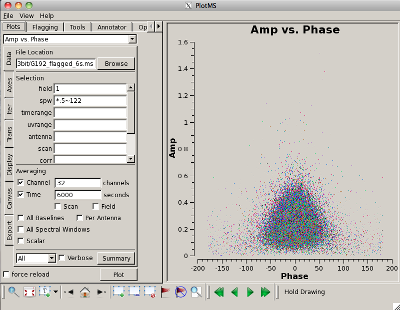
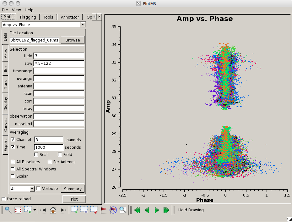
As always, it's a good idea to check the corrected data with plotms. Plots of corrected amplitude vs. baseline:
# In CASA
plotms(vis='G192_flagged_6s.ms', field='0', \
       xaxis='baseline', yaxis='amp', \
       ydatacolumn='corrected', spw='*:5~122', \
       averagedata=True, avgchannel='8', \
       avgtime='1000s', coloraxis='antenna1')
#
plotms(vis='G192_flagged_6s.ms', field='1', \
       xaxis='baseline', yaxis='amp', \
       ydatacolumn='corrected', spw='*:5~122', \
       averagedata=True, avgchannel='32', \
       avgtime='6000s', coloraxis='antenna1')
#
plotms(vis='G192_flagged_6s.ms', field='3', \
       xaxis='baseline', yaxis='amp', \
       ydatacolumn='corrected', spw='*:5~122', \
       averagedata=True, avgchannel='8', \
       avgtime='1000s', coloraxis='antenna1')
And, finally, corrected amplitude vs. corrected phase:
# In CASA
plotms(vis='G192_flagged_6s.ms', field='0', \
       xaxis='phase', yaxis='amp', \
       xdatacolumn='corrected', \
       ydatacolumn='corrected', spw='*:5~122', \
       averagedata=True, avgchannel='8', \
       avgtime='1000s', coloraxis='baseline')
#
plotms(vis='G192_flagged_6s.ms', field='1', \
       xaxis='phase', yaxis='amp', \
       xdatacolumn='corrected', \
       ydatacolumn='corrected', spw='*:5~122', \
       averagedata=True, avgchannel='32', \
       avgtime='6000s', coloraxis='baseline')
#
plotms(vis='G192_flagged_6s.ms', field='3', \
       xaxis='phase', yaxis='amp', \
       xdatacolumn='corrected', \
       ydatacolumn='corrected', spw='*:5~122', \
       averagedata=True, avgchannel='8', \
       avgtime='1000s', coloraxis='baseline')
Everything looks good, and the recalibration made only minor adjustments since there wasn't very much additional flagged data.
Now, split off the data for the calibrators and target field into separate MSs, so we can restore easily our calibrated dataset in case issues with data corruption arise. Before running split each time, we will remove any existing split data with the same name. Split will not automatically overwrite an existing MS. The inputs are:
# In CASA: splitting calibrated data 3C147
rmtables('3C147_split_6s.ms')
split(vis='G192_flagged_6s.ms', outputvis='3C147_split_6s.ms', \
      datacolumn='corrected', field='0')
# In CASA: splitting calibrated data J0603+174
rmtables('J0603_split_6s.ms')
split(vis='G192_flagged_6s.ms', outputvis='J0603_split_6s.ms', \
      datacolumn='corrected', field='1')
# In CASA: splitting calibrated data G192
rmtables('G192_split_6s.ms')
split(vis='G192_flagged_6s.ms', outputvis='G192_split_6s.ms', \
      datacolumn='corrected', field='2')
# In CASA: splitting calibrated data 3C84
rmtables('3C84_split_6s.ms')
split(vis='G192_flagged_6s.ms', outputvis='3C84_split_6s.ms', \
      datacolumn='corrected', field='3')
We can now move on to imaging!
Imaging
The G192 data were taken in the VLA's highest-resolution A-configuration at Ka-band. To determine the best parameters for imaging, it helps to start with the relevant information in the Observational Status Summary:
- The synthesized beam is expected to be ~0.059" at 33 GHz with a primary beam field-of-view of 1.4 arcmin (82").
Our data spans 27.0-38.4 GHz: this is a relatively very large fractional bandwidth (about 35%), resulting in substantial variation of the field of view over the entire frequency range. The FOV = 45 arcmin / Frequency (GHz), giving 1.7 arcmin at 27 GHz and 1.2 arcmin at 38.4 GHz. Likewise, the synthesized beam ranges from 0.072" at 27 GHz to 0.051" at 38.4 GHz. We want to subsample the synthesized beam by a factor of 3-5, so we will use a cellsize of 0.015". To cover the full FOV, we would want a minimum image size of 6800 pixels. However, there isn't much outside the center of the field for G192 -- this is what gave us leeway to average to 6 seconds -- so, to save time, we will only image a 1280x1280 pixel field (19.2"x19.2").
We will also use the Briggs robust (with robust=0.5) weighting, which is a compromise between uniform and natural weighting. Briggs weighting will produce an image with a reasonable resolution, but will allow us to still see larger scale structure. Noise from sidelobes will also be reduced compared to Natural weighting.
Due to the numerology of FFTW's (which clean uses under the hood for FFTs) optimal sizes, imsize should be an even number with prime factors chosen from 2, 3, 5, and 7. Since 1280 = (2^8)*5, it will give us optimal clean performance. Note that clean will still run if imsize does not have prime factors 2, 3, 5, or 7 (it will just be a bit slower) but you should always choose an even number.
For more information on using clean, in particular on using the interactive GUI, see EVLA_Continuum_Tutorial_3C391#Initial_Imaging.
NOTE: If you are pressed for time, then you might want to jump ahead to cleaning both basebands, and while it is cleaning you can read the other Imaging descriptions.
Cleaning a single spectral window
Let us start by interactively cleaning one spectral window in the lower-frequency baseband (spw 48). (For Ka-band, the higher-numbered spectral-window baseband is actually the lower-frequency baseband.)
Note that interrupting clean by Ctrl+C may corrupt your visibilities -- you may be better off choosing to let clean finish. We are working on a way to prevent this from happening, but for the moment it's best to avoid Ctrl+C.
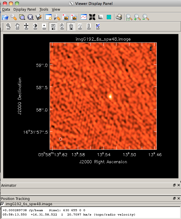
# In CASA: single spectral window cleaning
# Removing any previous cleaning information
# This assumes you want to start this clean from scratch
# If you want to continue this from a previous clean run,
# the rmtables command should be be skipped
rmtables('imgG192_6s_spw48*')
clean(vis='G192_split_6s.ms', spw='48:5~122', \
      imagename='imgG192_6s_spw48', \
      mode='mfs', nterms=1, niter=10000, \
      imsize=[1280], cell=['0.015arcsec'], \
      imagermode='csclean', cyclefactor=1.5, \
      weighting='briggs', robust=0.5, \
      interactive=True)
- Click on the wrench icon
 to bring up the Data Display Options and change the color scale to "Hot Metal 1" under "basic settings"
 - Zoom in 4 times
- Draw a box the point-like source and double-click inside the box to set your clean box (or clean "mask")
Change the number of iterations on the upper left to 50. (Note: this number is independent from the niter clean parameter, which applies to cleaning in mode interactive = False and is used if you click the right-pointing arrow button on the upper right to continue cleaning non-interactively.)
- The curved arrow on the upper right should now be highlighted in green. Click this green icon to clean the boxed source.
- Stop cleaning when the residuals look like the noise (this will probably happen after the first 50-100 iterations).
- To stop, click the red
 button.
When clean is finished, we can look at the restored image:
# In CASA
viewer('imgG192_6s_spw48.image')
The restored image is shown above.
Check the rms of the residuals using the imstat task:
# In CASA
mystat = imstat('imgG192_6s_spw48.residual')
print 'Residual standard deviation = '+str(mystat['sigma'][0]) + ' Jy'
In this particular case, it's 136 uJy; yours may be slightly different.
Cleaning the lower-frequency baseband
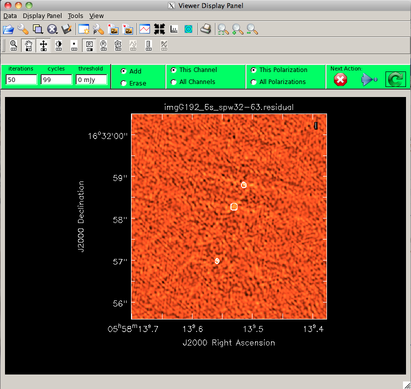
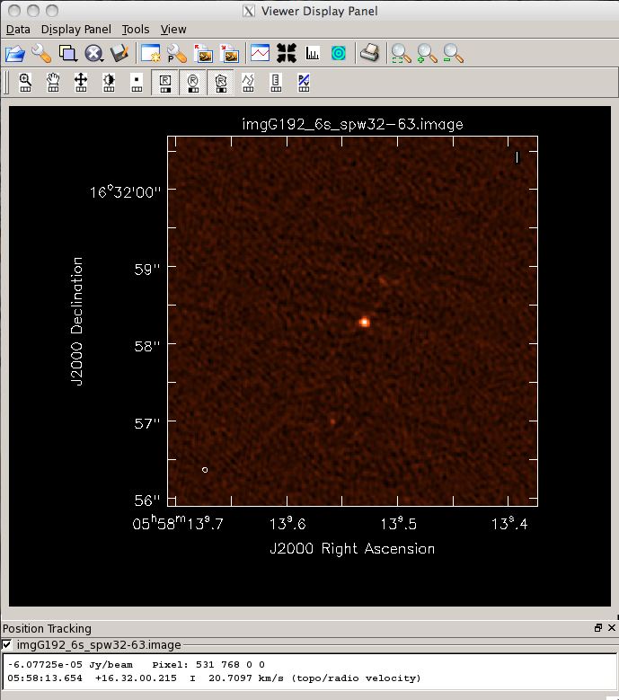
Here we will image the entire lower-frequency baseband (spw 32-63). Follow the same iterative procedure as before, and get the best residuals you can without "cleaning the noise".
# In CASA: lower frequency baseband cleaning
# Removing any previous cleaning information
# This assumes you want to start this clean from scratch
# If you want to continue this from a previous clean run,
# the rmtables command should be be skipped
rmtables('imgG192_6s_spw32-63*')
clean(vis='G192_split_6s.ms', spw='32~63:5~122', \
      imagename='imgG192_6s_spw32-63', \
      mode='mfs', nterms=1, niter=10000, \
      imsize=[1280], cell=['0.015arcsec'], \
      imagermode='csclean', cyclefactor=1.5, \
      weighting='briggs', robust=0.5, \
      interactive=True)
#
viewer('imgG192_6s_spw32-63.image')
mystat = imstat('imgG192_6s_spw32-63.residual')
print 'Residual standard deviation = '+str(mystat['sigma'][0]) + ' Jy'
- Because of the increased bandwidth, it is easier to see two fainter point sources.
- Be careful cleaning sources that lie near or on sidelobe peaks.
- Clean the central emission region first (50 iterations) to reduce the sidelobe level before adding any more components. The screenshot above shows the interactive clean window after 50 iterations with the three clean boxes we created.
For this run, the rms is 23 uJy. To the right is a zoom-in on the center of the restored image.
Finally, we will fit the central point source to determine its flux. First, create a box region around the source in the viewer, and save it as G192.crtf (View -> Regions -> File; see the screenshot below right). Note that you can drag the Regions window out of the main Viewer window if it's taking up too much space.
Use this region to fit the source flux:
# In CASA
myfit = imfit('imgG192_6s_spw32-63.image', region='G192.crtf')
print 'Source flux = '+str(myfit['results']['component0']['flux']['value'][0])+'+/-'+str(myfit['results']['component0']['flux']['error'][0]) + ' Jy'
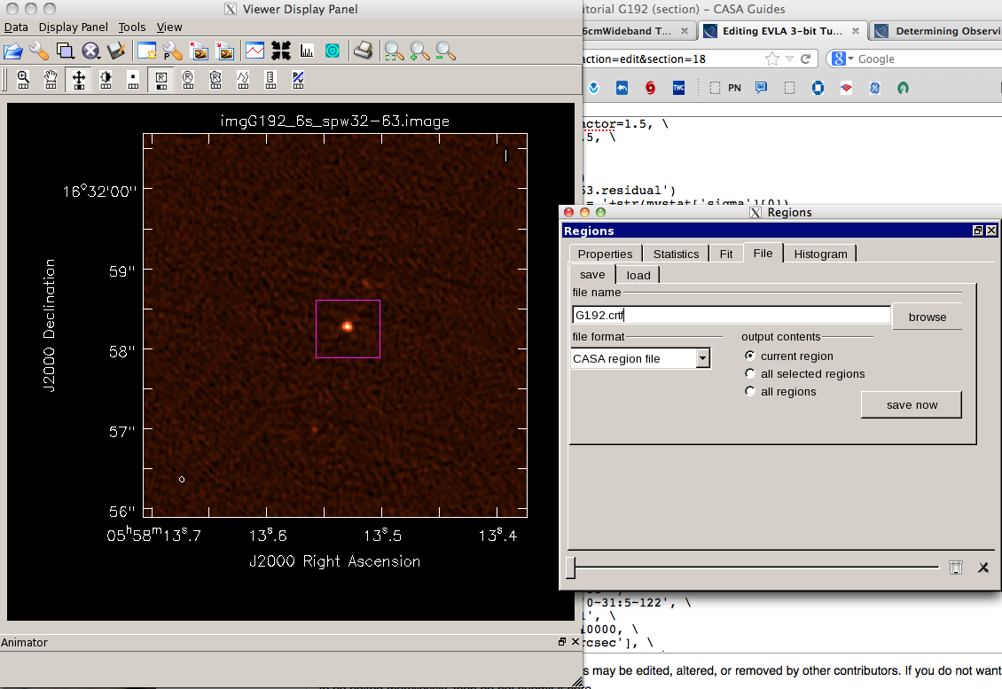
The derived flux is 2.64 +/- 0.04 mJy. Also, have a look at the logger output:
Image component size (convolved with beam) ---
       --- major axis FWHM:     80.01 +/- 0.98 marcsec
       --- minor axis FWHM:     71.51 +/- 1.01 marcsec
       --- position angle: 63.2 +/- 2.2 deg

Clean beam size ---
       --- major axis FWHM: 0.06 arcsec
       --- minor axis FWHM: 0.06 arcsec
       --- position angle: 29.00 deg
Image component size (deconvolved from beam) ---
       --- major axis FWHM:     51.3 +/- 1.8 marcsec
       --- minor axis FWHM:     37.7 +/- 2.3 marcsec
       --- position angle: 78.5 +/- 6.3 deg
The deconvolved size of around 51.3 x 37.7 milliarcseconds corresponds to a size of roughly 90 AU (assuming a distance of approximately 2 kpc). Indeed, this is thought to be the accretion disk around the protostar! (See this article for the initial report, using 43 GHz data, of the accretion disk around G192.)
Cleaning the upper-frequency baseband
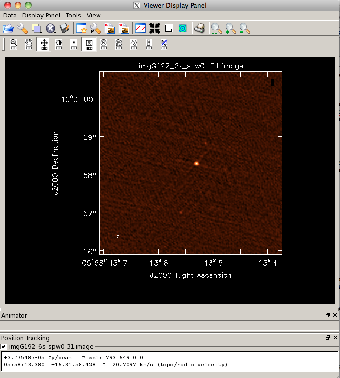
Now we will image the entire upper-frequency baseband (spw 0-31). Follow the same iterative procedure as before, and get the best residuals you can without "cleaning the noise".
# In CASA: upper frequency baseband cleaning
# Removing any previous cleaning information
# This assumes you want to start this clean from scratch
# If you want to continue this from a previous clean run,
# the rmtables command should be be skipped
rmtables('imgG192_6s_spw0-31*')
clean(vis='G192_split_6s.ms', spw='0~31:5~122', \
      imagename='imgG192_6s_spw0-31', \
      mode='mfs', nterms=1, niter=10000, \
      imsize=[1280], cell=['0.015arcsec'], \
      imagermode='csclean', cyclefactor=1.5, \
      weighting='briggs', robust=0.5, \
      interactive=True)
#
viewer('imgG192_6s_spw0-31.image')
mystat = imstat('imgG192_6s_spw0-31.residual')
print 'Residual standard deviation = '+str(mystat['sigma'][0]) + ' Jy'
myfit = imfit('imgG192_6s_spw0-31.image', region='G192.crtf')
print 'Source flux = '+str(myfit['results']['component0']['flux']['value'][0])+'+/-'+str(myfit['results']['component0']['flux']['error'][0]) + ' Jy'
For this run, the rms is 31 uJy, and the source flux is 3.07 +/- 0.06 mJy. Again, imfit finds that the source is slights extended and provides a deconvolved size. To the right is a zoomed-in image of the center of the restored image.
Cleaning both basebands using two MFS Taylor terms
From the individual images of the upper- and lower-frequency basebands, we can see that the source spectrum of G192 is relatively flat, with a spectral index of approximately
[math]\displaystyle{ \alpha = \log(S_1 / S_2) / \log(\nu_1 / \nu_2) }[/math] [math]\displaystyle{ = \log(3.07 / 2.64) / \log(36.5 / 29.0) }[/math] [math]\displaystyle{ = 0.66, }[/math]
where the convention for the spectral index alpha is that
[math]\displaystyle{ S \propto \nu^\alpha. }[/math]
Within a single baseband, neglecting to account for the spectral index will make little difference -- however, when we combine the two basebands, it is best to account for the spectral variation across the total band. For this, we will set nterms=2 in clean.
This option creates two "Taylor term" images -- an average intensity image (with suffix .image.tt0), and a spectral slope image (with suffix .image.tt1), which is intensity x alpha (where alpha is the spectral index). For convenience, there is also a spectral index image (with suffix .image.alpha). These Taylor expansions are with respect to the "reference frequency" of the image (by default the center frequency of the selected spectral window, but can be specified using the reffreq parameter in clean).
We will clean the complete dataset using nterms=2. Note: if you prefer, you can clean your image using interactive = False. For non-interactive cleaning, make sure you define a clean mask with mask='imgG192_6s_spw0-31.mask' or mask='imgG192_6s_spw32-63.mask' to use these as a starting point rather than running an interactive clean session. You can also draw a new region file from scratch in the Viewer, save the region as a .crtf file, and supply this file to the mask parameter in clean. If you set interactive = False you should also modify the threshold and niter parameters to avoid over-cleaning (the threshold parameter should always be higher than the expected theoretical rms noise; for an estimation of the rms noise for this image see below).
# In CASA: basebands mfs taylor cleaning
# Removing any previous cleaning information
# This assumes you want to start this clean from scratch
# If you want to continue this from a previous clean run,
# the rmtables command should be be skipped
rmtables('imgG192_6s_spw0-63_mfs2*')
clean(vis='G192_split_6s.ms', spw='0~63:5~122', \
      imagename='imgG192_6s_spw0-63_mfs2', \
      mode='mfs', nterms=2, niter=10000, gain=0.1, \
      threshold='0.0mJy', psfmode='clark', imsize=[1280], \
      cell=['0.015arcsec'], \
      weighting='briggs', robust=0.5, interactive=True)
#
mystat = imstat('imgG192_6s_spw0-63_mfs2.residual.tt0')
print 'Residual standard deviation = '+str(mystat['sigma'][0]) + ' Jy'
myfit = imfit('imgG192_6s_spw0-63_mfs2.image.tt0', region='G192.crtf')
print 'Source flux = '+str(myfit['results']['component0']['flux']['value'][0])+'+/-'+str(myfit['results']['component0']['flux']['error'][0]) + ' Jy'
For this run, the rms is 19.7 uJy, and the peak of the emission from G192 is 1.8 mJy, and the integrated source flux is 2.86 +/- 0.04 mJy (as before, the source is found to be extended). You can use the viewer to load the average intensity image:
# In CASA
viewer('imgG192_6s_spw0-63_mfs2.image.tt0')

Since the spectral index image is very noisy in the lower-intensity regions, we will use immath task to filter the spectral index image explicitly, using a Lattice Expression Language (LEL) expression:
# In CASA: spectral index image filtering
immath(imagename=['imgG192_6s_spw0-63_mfs2.image.alpha',
                  'imgG192_6s_spw0-63_mfs2.image.tt0'], \
       mode='evalexpr', \
       expr='IM0[IM1>2.0E-4]', \
       outfile='imgG192_6s_spw0-63_mfs2.image.alpha.filtered')
This will use 0.2 mJy (10 x the rms) as the cutoff. You can then view or manipulate the filtered alpha image as usual.
We can also use LEL to filter the alpha image on intensity on-the-fly when we load the raster via the Open Data panel, by specifying a LEL string in the LEL box instead of selecting the image from the directory listing. The LEL string
'imgG192_6s_spw0-63_mfs2.image.alpha'['imgG192_6s_spw0-63_mfs2.image.tt0'>2E-04]
will replicate what we did above. The middle figure to the right shows the Open Data panel with our LEL string in it. Just click the Raster button to load this.
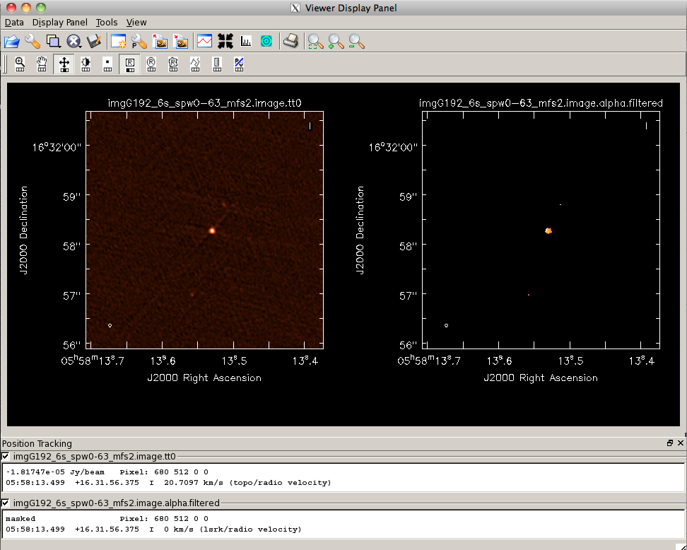
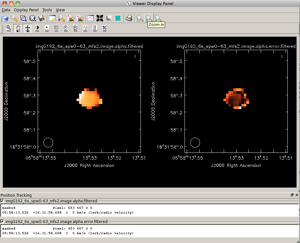
The lower panel to the right shows the intensity and LEL-filtered alpha images side-by-side in the viewer, zoomed in on the brightest source of emission. Creating a box around this region and double-clicking reveals that the spectral index varies from around -0.33 to 1.4, with the pixels in the brightest portion of the image at around 0.8, similar to what we found by hand using the information from the single-baseband images.
To get a sense of the probable errors for this spectral index information, we perform a similar filtering operation on the imgG192_6s_spw0-63_mfs2.image.alpha.error>/tt> image:
# In CASA: spectral index probable errors filtering
immath(imagename=['imgG192_6s_spw0-63_mfs2.image.alpha.error',
                  'imgG192_6s_spw0-63_mfs2.image.tt0'], \
       mode='evalexpr', \
       expr='IM0[IM1>2E-4]', \
       outfile='imgG192_6s_spw0-63_mfs2.image.alpha.error.filtered')
Now, we can load both the alpha and alpha.error images side-by-side in the viewer:
# In CASA
viewer('imgG192_6s_spw0-63_mfs2.image.alpha.filtered')
As one might expect, the errors are higher outside the emission peak (see the screenshot on the right). However, it seems possible that the .error image is underestimating the true errors on the mfs-calculated spectral index, since the central brightest pixels only have errors of around 0.15, when we calculated an alpha of 0.66 (compared with the mfs-calculated alpha of 0.8). If we were planning to use the reported spectral index information for publication, we would need to go through a more thorough investigation of the actual error analysis and spectral index.
Analyzing the image
From imstat on the final combined-baseband image, we got an image rms of 19.7 uJy. A reasonable question to ask is what we would expect the image rms to be: one way to estimate this is to determine the effective on-source time, then input the appropriate parameters to the VLA exposure calculator to determine the expected rms.
# In CASA
listobs('G192_split_6s.ms', listunfl=True)
This will show:
ID   Code Name                RA               Decl           Epoch   SrcId      nRows    nUnflRows
0    NONE G192.16-3.84        05:58:13.540000 +16.31.58.30001 J2000   0        2931890   2901697.32
Note that the "nUnflRows," or number of unflagged rows, is 2901697.32. Every row is a single baseline-integration-spw record, as you probably learned if you looked at the MS with browsetable. So, to use this to calculate an "effective" exposure time for the VLA Exposure Calculator for 22 antennas (22*21/2 = 231 baselines), we find that time = 2901697.32 * 6 seconds / 231 baselines / 64 spectral windows = 1178 seconds = 19.6 minutes. Our effective bandwidth is 7552 MHz, taking into account the spectral window selection. Using the median frequency of 32.7 GHz, the VLA exposure calculator reports that we should achieve an image rms of 13.5 uJy. Although our actual rms is somewhat higher, this is not unexpected; we have not done any self-calibration, for example.
Next, we will do some rough analysis on the spectral index to determine an intensity-weighted mean spectral index for G192. The .image.tt1 from our mfs is an intensity times alpha image (see the figure to the right). Let's filter this Taylor-term image by intensity as we did with the .alpha image:
# In CASA: intensity weighted mean spectral analysis
# Removing any file output from previous runs, so immath will proceed
rmtables('imgG192_6s_spw0-63_mfs2.image.tt1.filtered')
immath(imagename=['imgG192_6s_spw0-63_mfs2.image.tt1',
                  'imgG192_6s_spw0-63_mfs2.image.tt0'], \
       mode='evalexpr', \
       expr='IM0[IM1>2E-4]', \
       outfile='imgG192_6s_spw0-63_mfs2.image.tt1.filtered')
#
# Removing any file output from previous runs, so immath will proceed
rmtables('imgG192_6s_spw0-63_mfs2.image.tt0.filtered')
immath(imagename=['imgG192_6s_spw0-63_mfs2.image.tt0'], \
       mode='evalexpr', \
       expr='IM0[IM0>2E-4]', \
       outfile='imgG192_6s_spw0-63_mfs2.image.tt0.filtered')
We can use the same region we created for imstat. Let us compute the intensity-weighted spectral index over this region by averaging these masked images using imstat and computing the ratio:
# In CASA
mystat = imstat('imgG192_6s_spw0-63_mfs2.image.tt1.filtered', \
                region='G192.crtf')
avgtt0alpha = mystat['mean'][0]
#
mystat = imstat('imgG192_6s_spw0-63_mfs2.image.tt0.filtered', \
                region='G192.crtf')
avgtt0 = mystat['mean'][0]
avgalpha = avgtt0alpha / avgtt0
print 'G192 intensity-weighted alpha = ' + str(avgalpha)
We get:
G192 intensity-weighted alpha = 0.737300481129
This is pretty close to the value we found from the single-baseband images of alpha = 0.66, validating the results from mfs with nterms=2.
What to do next: some exercises for the user
Here are a number of things you can try after completing this tutorial:
- Use self-calibration to improve the data and re-clean to make a better image. See this tutorial for more information on self-calibration.
- Investigate the data further to see if any more flagging is needed.
- Image the calibrators. What sort of dynamic range can you get on them? Is self-calibration needed (and if so what dynamic range do you get when you use it)?
- Try the rflag algorithm in the flagdata task to automatically flag bad data based on the statistics of the data (though there is not much left, really). There is more information on running the rflag algorithm in this tutorial.
Credits
The Jansky Very Large Array (VLA) is a partnership of the United States, Canada, and Mexico. The VLA is funded in the United States by the National Science Foundation, in Canada by the National Research Council, and in Mexico by the Comisión Nacional de Investigación Científica y Tecnológica (CONICyT).
The National Radio Astronomy Observatory is a facility of the National Science Foundation operated under cooperative agreement by Associated Universities, Inc.
Last checked on CASA Version 4.4.0.