ADMIT Products and Usage CASA 6
Most recently updated for CASA Version 6.6.1 using Python 3.8
Intro/What is ADMIT?
The ALMA Data-Mining Toolkit (ADMIT) was developed by The ADMIT Team at UMD as an ALMA Development Project delivered in 2016.
ADMIT is an execution environment and set of tools for analyzing image data cubes. ADMIT is based on python and designed to be fully compliant with CASA and to utilize CASA routines where possible. ADMIT has a flow-oriented approach, executing a series of ADMIT Tasks (AT) in a sequence to produce a sequence of outputs. For the beginner, ADMIT can be driven by simple scripts that can be run at the Unix level or from inside of CASA. ADMIT provides a simple browser interface for looking at the data products, and all major data products are on disk as CASA images and graphics files. For the advanced user, ADMIT is a python environment for data analysis and for creating new tools for analyzing data.
For a detailed quick-look at ALMA images, standardized ADMIT “recipes” can be run which produce various products depending on the image type. For continuum images, ADMIT simply finds some of the basic image properties (RMS, peak flux, etc) and produces a moment map. For cube images, ADMIT will analyze the cube, attempt to identify spectral features, and create moment maps of each identified spectral line.
ADMIT does not interact with u,v data or create images from u,v data; CASA should be used to create images. ADMIT provides a number of ways to inspect your image cubes. The astronomer can then decide whether the ALMA image cubes need to be improved, which requires running standard CASA routines to re-image the u,v data. If new images are made, the ADMIT flow can be run on these new image cubes to produce a new set of ADMIT products.
Obtaining ADMIT and data for this guide
For this CASA Guide, we will go through creating an ADMIT product of some science verification data and then inspect the output. You’ll of course need CASA installed (http://casa.nrao.edu/casa_obtaining.shtml) as well as ADMIT. To install ADMIT from scratch for use in CASA 6, you’ll need to clone the source code using git and then edit the setup script to create the necessary environment. Note that matplotlib and scipy are required for installation.
# In bash

# python3.8 -m pip install --user matplotlib
# python3.8 -m pip install --user scipy

# cd to the directory you want to host ADMIT in
git clone https://github.com/astroumd/admit
cd admit
git checkout python3
pip install -e .
If the pip command does not work, try using pip3 or python3 -m pip install -e .
This will set up your ADMIT installation to run with Python 3 and be compatible with CASA 6. After running the above commands, you'll need to edit the admit_start.sh.in startup file. The default file with comments about what parameters to edit appear below. The PATH, TCL_LIBRARY, and TK_LIBRARY variables have already been edited from the default values to the required values.
# @EDIT_MSG@
# for (ba)sh : source this file

export  ADMIT=@ADMIT@          # This needs to match the path of your ADMIT installation, i.e. the current directory
export  CASA_ROOT=@CASA_ROOT@  # This should be the path to your CASA installation. Do NOT include /bin, which is added below.
if test "x$CASA_ROOT" = "x"; then
    unset CASA_ROOT
    export PATH=${ADMIT}/bin:${PATH}
else
    # CASA_ROOT has been deprecated as a bin by CASA
    export PATH=${ADMIT}/bin:${CASA_ROOT}/bin:${CASA_ROOT}/lib/casa/bin:${CASA_ROOT}/:${PATH}
    export TCL_LIBRARY=${CASA_ROOT}/share/tcl
    export TK_LIBRARY=${CASA_ROOT}/share/tk
    export LD_LIBRARY_PATH=${CASA_ROOT}/lib:${LD_LIBRARY_PATH}
fi

export CASA_PATH="$CASA_ROOT linux admit `hostname`"

export PYTHONPATH=${ADMIT}:${PYTHONPATH}
Once you have edited the configuration script, simply source the admit_start.sh.in script before executing any ADMIT commands.
# In bash
source admit_start.sh.in
If you want to check that ADMIT is set up, you can type
# In bash
admit
ADMIT        = <your/ADMIT/installation/path>
    version  = 1.0.8.6
CASA_PATH   = <your/CASA/installation/path> linux admit <pc-name>
CASA_ROOT    = <your/CASA/installation/path>
    prefix   = <ERROR>
    version  = <ERROR>
    revision = <ERROR>
Trying CASA6, no worries if this fails
The casa-config file previously found in /bin for CASA 5 is now deprecated in CASA 6, resulting in the errors above. ADMIT should run ok regardless.

If the admit command returns an error below the "Trying CASA6" output, this is also ok. The error is usually just from a mixup in the metadata bookkeeping.
In your terminal after sourcing the start script you should see the directory paths and versions of ADMIT. For more details, please see the ADMIT installation guide.
Now switch directories out of the ADMIT installation you just set up and to where you will be working on the data. For this guide, we’ll be using the images generated from the AntennaeBand7 CASA Guide. We just need the reference images which we can download with wget and then untar. Follow the link in AntennaeBand7#Obtaining_the_Data to the most recent image products.
# In bash
cd <working_dir>
wget <link/to/most/recent>/Antennae_Band7_ReferenceImages.tgz
tar xzfv Antennae_Band7_ReferenceImages.tgz
cd Antennae_Band7_ReferenceImages # if this exists
Creating an ADMIT product
Now that we have some ALMA images and ADMIT installed, let’s run one of the standard ADMIT recipes on our image. There are two standard recipes that handle most ALMA images:
The AntennaeBand7 images are data cubes so we’ll use the first recipe. Call the admit1.py recipe which allows you to use flags for customization. To do this, type:
# In bash
runa1 Antennae_North.CO3_2Line.Clean.pcal1.image.fits
# or
</path/to/your/admit/installation>/admit/admit/test/admit1.py Antennae_North.CO3_2Line.Clean.pcal1.image.fits
Caveat: runa1 and runa2 might not work in CASA 6, in which case you should use the second method to specify the full path to admit1.py.
This will produce a long sequence of outputs in the terminal; however, there are over 30 tunable parameters that allow you to set the VLSR, rest frequency, regions of interest, etc. as well as many line identification parameters to tune such as using the online version of Splatalogue rather than the internal one for line identification. These can be tuned via creating a file with your parameter choices and specifying it via the --apar flag. Later in this guide we will go through a little bit more on how to customize ADMIT to better suit your data but for now, more information can be found in ADMIT Tricks.
In the end, if everything worked correctly, admit1.py will result in the creation of a file named Antennae_North.CO3_2Line.Clean.pcal1.image.admit which contains the output from the ADMIT recipe.
The ADMIT weblog, viewing the ADMIT product


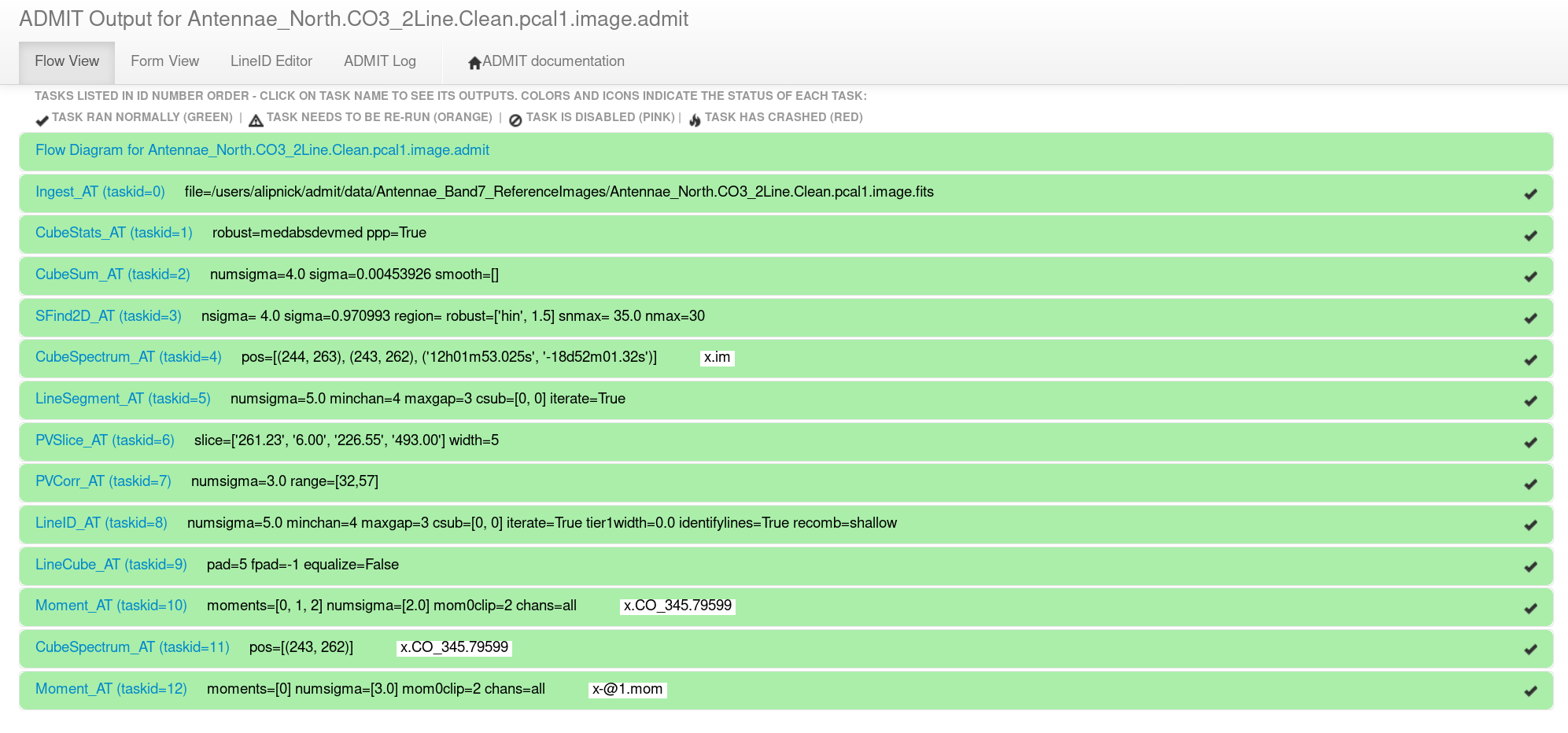
To view the ADMIT output, start by descending into the Antennae_North.CO3_2Line.Clean.pcal1.image.admit directory and open up the index.html file in your favorite browser (currently Firefox is the best option). This will open up the ADMIT browser interface (weblog) which is the most convenient way to view the ADMIT results on the image. It should look something like Figure 1.
The text within each bar gives the ADMIT Task name, the task ID number, the parameters that were used within that task, and any output image names. Note that ADMIT uses the basename "x" if one isn't supplied so all the output file names will be "x.*". Clicking on one of the green horizontal bars will reveal all the output for that ADMIT task. Just under the expanded bar will be the task name (which hyperlinks to the ADMIT wiki page for that task) and a one-line explanation of what that task does (Figure 2).
Now, we will go through all of the output in the ADMIT weblog and describe what each task does and what output to expect.
The ADMIT Data Flow

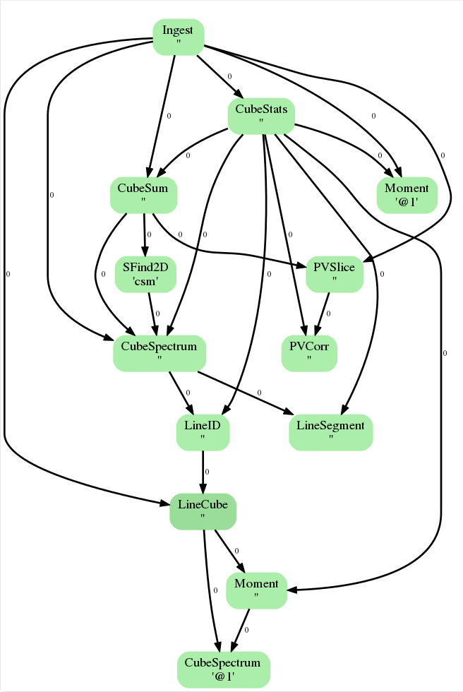
Clicking on the top-most bar of the weblog, “Flow Diagram for Antennae_North.CO3_2Line.Clean.pcal1.image.admit” (see Figure 1), reveals the “ADMIT Flow Diagram” (Figure 3). This is an illustration of how the products created in each task flow through the entire process. For a detailed discussion of how ADMIT flows work (and how to create your own) please see Workflow Management.
For continuum images, these diagrams are extremely simple but for line-dense image cubes these can be incredibly complicated. This diagram is a directed acyclic graph representing the ADMIT Task connections. Each arrow represents the connection from an ADMIT task output to the input of another ADMIT Task. The integer next to each arrow is the zero-based index of the ADMIT Task's output basic data product. Note that any output basic data product may be used as the input for more than one ADMIT Task.
Ingest_AT
This is the most basic task that is performed at the beginning of any ADMIT workflow. This task reads in a FITS image, creates a CASA image and extracts basic information such as rest frequency, beam size, image size, minimum/maximum values, etc.
CubeStats_AT
This task computes statistics on the image cube in the image-plane (meaning that the uv data is not examined). Here, ADMIT computes per-channel statistics in order to find the maximum and minimum values and pixel locations throughout the cube. This information is then used to generate global statistics such as mean intensity, a signal-free estimate of the noise, and the dynamic range. The maximum value pixel locations throughout the cube will also be used in later steps to help identify lines in the spectrum. Additionally, two plots are created:
- Emission Characteristics Plot: The spectrum of various statistical measures (SNR, peak signal, RMS, and minimum signal) are plotted.
- The Peak Point Plot: the image is searched and the peak emission locations are found for every channel in the cube and plotted. The size of the point in the image indicates the magnitude of the emission in that channel.
CubeSum_AT
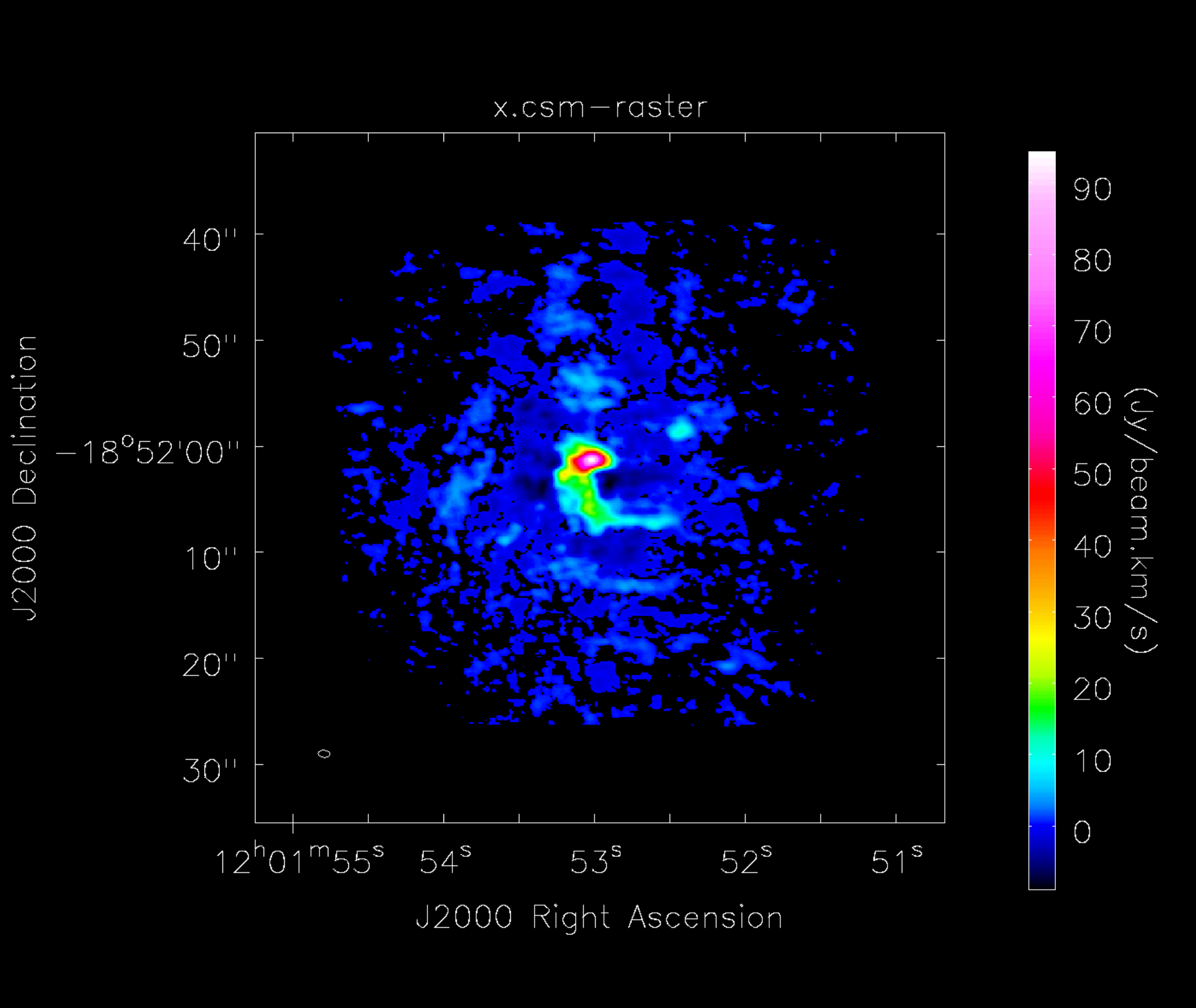
This task creates a moment 0 map of all the emission in the image cube, regardless of whether or not it comes from different spectral lines (Figure 4). The RMS, and therefore cutoff emission level, is determined by the previous step, CubeStats_AT.

SFind2D_AT
This task creates a list of sources found in the 2D image created by CubeSum_AT. The output is a table which lists peak source positions and fluxes. An image is also displayed which shows where the sources are located.
CubeSpectrum_AT
Given the input from SFind2D_AT of source positions, the statistics of the image from CubeStats_AT, the moment map created by CubeSum_AT, and the initial input image, this task computes the spectra of the cube at a specific point (or points). The output are averaged spectra taken at the locations of the three maximum flux values in the cube.
LineSegment_AT
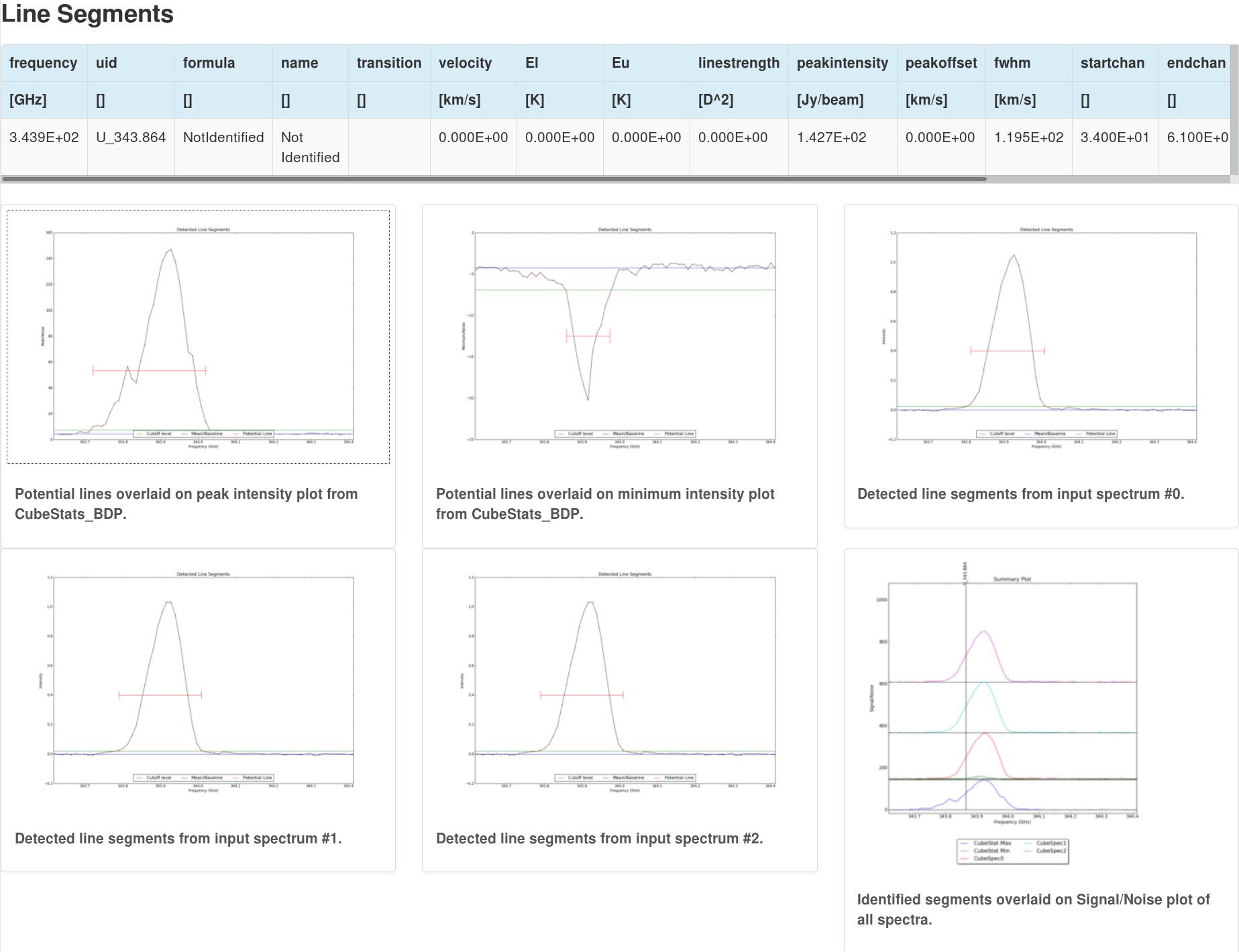
This task detects segments of emission (i.e. spectral lines) based on RMS cutoffs and the input spectra provided from the previous CubeSpectrum_AT task but does not yet identify the lines (this will be done in a later stage). The output is then a list of potential spectral lines as well as spectra showing where the potential lines have been identified. Six plots are created (see Figure 5): peak intensity, minimum intensity, the three spectra provided as inputs from CubeSpectrum_AT, and a Signal/Noise summary plot. For each spectrum, the potentially identified lines are overlaid and the amplitude is given as a multiple of the noise (either Peak/Noise or Minimum/Noise).

PVSlice_AT
This task creates a position-velocity (PV) diagram through the input image cube. Given the original image cube and the output moment map from CubeSum_AT, the moment of inertia is computed and used to derive "the best slice" through the image cube. The output is then two figures; the location of the PV slice drawn through the moment map, and the PV diagram.
PVCorr_AT
Using an input PV slice from PVSlice_AT and the cube statistics from CubeStats_AT (from which the RMS is taken), this task computes a cross-correlation of the PV slice. It does this by attempting to correlate sections of the spectrum with the whole PVSlice. If the section is not random noise, then the output will show a high correlation for that section. This can be most useful for detecting weak spectral lines.
LineID_AT
In this task, ADMIT identifies spectral lines in the input datacube using the output from CubeSpectrum_AT and CubeStats_AT. The output here is very similar to the above LineSegment_AT task except that the line segments have now been identified. For our example here of the Antenna North we see that the large spectral line has been correctly identified as CO (3-2).
LineCube_AT
Given the output list of lines from LineID_AT, this task generates smaller line cubes from the input image cube, each centered around an identified line. A table is presented showing the identified line molecule and rest frequency, the starting and ending channel for the smaller cube, and the name given to the output cube.
Moment_AT
For each line cube that is made during the above task, LineCube_AT, a moment map is produced via Moment_AT. This task uses the input line cube as well as information from CubeStats_AT to create a Moment 0, Moment 1, and Moment 2 map (Figure 6).

CubeSpectrum_AT
Likewise, for each line cube that is made during LineCube_AT, this task computes the spectrum for the pixel with the maximum flux value in the moment 0 map created by the Moment_AT task.
Moment_AT
Finally, ADMIT creates another moment 0 map using the full, original input cube and information from CubeStats_AT.
Customizing ADMIT for your dataset
As outlined near the beginning of this guide, you can customize an ADMIT run by supplying additional parameters to admit1.py via a parameter file and pointing to it with the --apar flag in your admit1.py call.
Each time ADMIT runs, it creates an admit0.py script (found in the same directory as the index.html file) which is an auto-generated script of the ADMIT flow that was performed. Therefore, another option for customizing your ADMIT output is to edit this script (admit0.py) to include extra parameters for your data, and run again.
For example, you may add the VLSR to Ingest_AT or LineID_AT for more accurate line identification, or you may change the “online” boolean flag in LineID_AT to “True” so that ADMIT searches the online version of Splatalogue to identify lesser known chemical species.
Example admit0.py:
#!/usr/bin/env casarun
#
# This script was auto-generated by ADMIT version 1.0.8.6 and may be overwritten;
# copy before editing. It expects to run from <working_dir>.
# If you need to start from scratch:   rm -rf Antennae_North.CO3_2Line.Clean.pcal1.image.admit
#
# This flow processes a single data cube. To process other cubes in the same
# way, call this script with another cube file as the command line argument:
# % admit0.py CUBEFILE
#
import os, sys
import admit

# Command line processing.
argv = admit.utils.casa_argv(sys.argv)
if len(argv) < 2:
  cubefile = 'Antennae_North.CO3_2Line.Clean.pcal1.image.fits'
  projdir = 'Antennae_North.CO3_2Line.Clean.pcal1.image.admit'
else:
  cubefile = argv[1]
  projdir = os.path.splitext(argv[1])[0] + '.admit'

# Master project.
p = admit.Project(projdir, commit=False)

# Flow tasks.
t0  = p.addtask(admit.Ingest_AT(basename='x', file=cubefile))
t1  = p.addtask(admit.CubeStats_AT(ppp=True), [t0])
t2  = p.addtask(admit.CubeSum_AT(numsigma=4.0, sigma=99.0), [t0, t1])
t3  = p.addtask(admit.Moment_AT(mom0clip=2.0, numsigma=[3.0]), [t0, t1])
t4  = p.addtask(admit.SFind2D_AT(alias='csm', numsigma=4.0, sigma=1.0810286980861303), [t2])
t5  = p.addtask(admit.PVSlice_AT(clip=2.0, pvsmooth=[10, 10], width=5), [t0, t2])
t6  = p.addtask(admit.CubeSpectrum_AT(), [t0, t1, t2, 'csm'])
t7  = p.addtask(admit.PVCorr_AT(), [t5, t1])
t8  = p.addtask(admit.LineSegment_AT(csub=[0, 0]), [t6, t1])
t9  = p.addtask(admit.LineID_AT(csub=[0, 0], references='etc/tier1_lines.list'), [t6, t1])
t10 = p.addtask(admit.LineCube_AT(), [t0, t9])
t11 = p.addtask(admit.Moment_AT(mom0clip=2.0, moments=[0, 1, 2]), [t10, t1])
t12 = p.addtask(admit.CubeSpectrum_AT(), [t10, t11])

# Update project.
p.run()
To find out what parameters are available for customization, please see the online documentation for each task by clicking on the task name under its header in the weblog.
It is best practice to first make a copy of the admit0.py script in your working directory (one directory above the <image_name>.admit directory). Then, edit and run this script to create the new ADMIT products:
# In bash
python3 admit0.py
Once you are comfortable with editing the admit0.py script, this can help you start to create your own ADMIT flows which you can use to help you quickly sift through large datasets.
Version History
If you would like to use the older, Python2 version of ADMIT with CASA 5, please instead follow the older version of this guide:
However, this is not recommended on modern systems due to the ongoing deprecation of both Python2 and CASA 5; the old instructions are made available for surviving older systems.