EVLA high frequency Spectral Line tutorial - IRC+10216-CASA4.5
Please use CASA 4.5 for this tutorial
Overview
This tutorial describes the data reduction for two spectral lines observed toward the Asymptotic Giant Branch (AGB) star IRC+10216. In this Jansky VLA OSRO1 mode observation, one subband (spectral window) was observed in each of the two basebands, with the subbands centered on the HC3N and SiS lines near 36 GHz. The raw data were loaded into CASA with importevla, where zero and shadowed data were flagged (note that this is done by the NRAO Data Archive). Then the data were split, so we could average from the native 1-second integrations to 10 seconds, selecting only antennas with Ka-band receivers and only spectral windows (called spw in CASA) with Ka-band data. This produces a significantly smaller data set for processing.
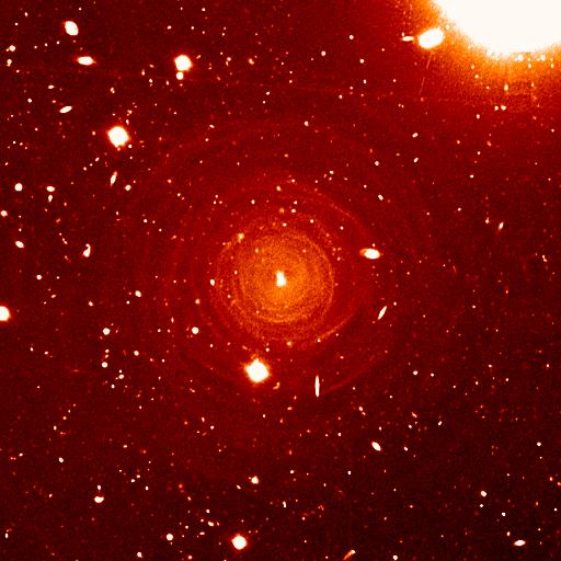
IRC+10216 (CW Leo) (see Figure 1) is the brightest star in the sky at 5 microns, but only 16th magnitude visually. It was discovered during the first survey of the infrared sky, carried out by Bob Leighton and Gerry Neugebauer in 1965. An Asymptotic Giant Branch star, it is a Mira-type variable going through prodigious episodic mass loss. The dust condensed from the atmosphere during the mass loss is responsible for the millimeter emission; the continuum emission, seen at radio wavelengths, probes the actual stellar photosphere. Molecules form along with the dust, and a steady state chemistry occurs in the dense inner regions (Tsuji 1973 A&A 23, 411). As the density of material drops, the chemistry freezes, but the molecules continue their long coast outward into the Galaxy. As the shell thins, ultraviolet light from the ambient galactic radiation field penetrates and initiates a new chemistry in the gas.
SiS, a simple molecule created in the dense inner envelope chemistry, is photodissociated as it coasts out into the shell. The result is the centrally condensed emission we see in the present observations. Interestingly, in the next lower transition at 18 GHz, the line shape is much different from what we see here. At the extreme velocities in the profile, very bright narrow emission is seen which has been interpreted as maser emission. The interested student can find VLA observations of this line in the NRAO Data Archive.
HC3N, a much more complex species, is created by the photochemistry which becomes active as atoms and pieces of molecules, destroyed by ultraviolet radiation, undergo the next phase of chemistry in the shell. HC3N has many vibrational modes, which may be excited, in addition to its rotational modes. Owing to this, it can re-radiate energy absorbed from ultraviolet radiation more effectively than some molecules with a single bond. Eventually, it too is destroyed; however, during its brief existence, its rise to abundance in the envelope results in a ring of emission, which is what is observed in this image made with the JVLA. A recent model by Cordiner & Millar (2009, ApJ, 697, 68) describes a new chemical model for the shell, which also takes into account the variation of mass loss by the star. They show that in addition to purely chemical effects, local gas and dust density peaks play a role in shaping the observed emission.
Obtaining the Data
The post-split averaged data can be downloaded from http://casa.nrao.edu/Data/EVLA/IRC10216/day2_TDEM0003_10s_norx.tar.gz (data size: 1.1GB)
We are providing this starting data set, rather than the true initial data set for at least two reasons. First, many of these initial processing steps can be rather time consuming (> 1 hr). Second, while necessary, many of these steps are not fundamental to the calibration and imaging process, which is the focus of this tutorial. For completeness, however, here are the steps that were taken from the initial data set to produce the starting data set.
If you want to start the data reduction from the beginning, from the NRAO Archive select the TDEM0003_sb1345754_1.55312.131578217595 data set.
- The initial Science Data Model (SDM) file was converted into a measurement set (MS).
- Basic data flagging was applied, to account for shadowing of the antennas. These data are from the D configuration, in which antennas are particularly susceptible to being blocked (shadowed) by other antennas in the array, depending upon the elevation of the source.
- The data were averaged from the initial 1-second correlator sample time to 10-second samples. In the D configuration, the fringe rate is relatively slow and time-average smearing is less of a concern.
All of these steps can be done directly from the NRAO Archive's Download page, by selecting CASA MS as the download format (it's a good idea to also check the Create MS or SDM tar file box), checking the Apply flags generated during observing box, and setting Time Averaging to 10s. Then, as noted above in the Overview, the Ka-band data for this source was split from the larger TDEM0003 MS to create the smaller data set that this tutorial covers.
Once the download is complete, unzip and unpack the file (within a working directory, which you will then run CASA):
# in a terminal, outside of CASA:
tar -xzvf day2_TDEM0003_10s_norx.tar.gz
How to Use This CASA Guide
There are a number of possible ways to run CASA, described in more detail in Getting Started in CASA. In brief, there are at least three different ways to run CASA:
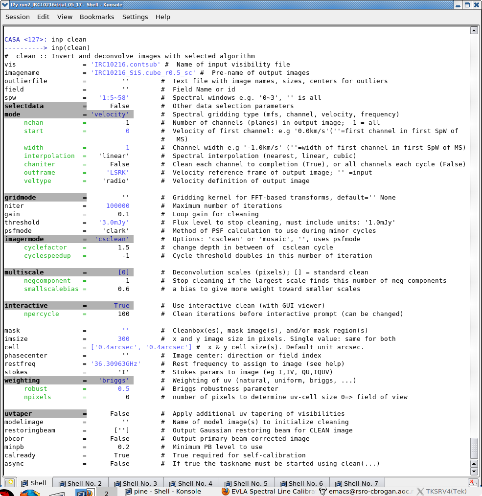
- Interactively examining task inputs. In this mode, one types taskname to load the task, inp to examine the inputs (see Figure 2), and go once those inputs have been set to your satisfaction. Allowed inputs are shown in blue and bad inputs are colored red. The input parameters themselves are changed one by one, e.g., selectdata=T. Screenshots of the inputs to various tasks used in the data reduction below are provided, to illustrate which parameters need to be set. More detailed help can be obtained on any task by typing help taskname. Once a task is run, the set of inputs are stored and can be retrieved via tget taskname; subsequent runs will overwrite the previous tget file.
- Pseudo-interactively via task function calls. In this case, all of the desired inputs to a task are provided at once on the CASA command line. This tutorial is made up of such calls, which were developed by looking at the inputs for each task and deciding what needed to be changed from default values. For task function calls, only parameters that you want to be different from their defaults need to be set.
- Non-interactively via a script. A series of task function calls can be combined together into a script, and run from within CASA via execfile('scriptname.py'). This and other CASA Tutorial Guides have been designed to be extracted into a script via the script extractor by using the method described at the Extracting scripts from these tutorials page. Should you use the script generated by the script extractor for this CASA Guide, be aware that it will require some small amount of interaction related to the plotting, occasionally suggesting that you close the graphics window and hitting return in the terminal to proceed. It is in fact unnecessary to close the graphics windows (it is suggested that you do so purely to keep your desktop uncluttered).
If you are a relative novice or just new to CASA, it is strongly recommended to work through this tutorial by cutting and pasting the task function calls provided below after you have read all the associated explanations. Work at your own pace, look at the inputs to the tasks to see what other options exist, and read the help files. Later, when you are more comfortable, you might try to extract the script, modify it for your purposes, and begin to reduce other data.
Initial Inspection and Flagging
Observing Logs
For all VLA observations, the operators keep an observing log. To can access the operator logs, go to the observing log website and enter a date range covering only 26 Apr 2010, then select TDEM0003. Pertinent information from this observation is repeated below:
INFORMATION FROM OBSERVING LOG:
Date of the observation: 26-April-2010
There are no Ka-band receivers on ea11, ea13, ea14, ea16, ea17, ea18, ea26
Antenna ea06 is out of the array
Antenna 15 has a focus timeout
Antennas ea10, ea12, ea22 do not have good baseline positions
All of that information we should keep in mind during the calibration, e.g., if the mentioned list of unavailable receivers do appear in the data, the data is just noise and should be flagged. For the data set that you have downloaded, the antennas have already been removed. Also, keep an eye on other messages such as loss of data, subreflector problems, or any other such issues. If they were not captured in the online flagging, they should be carefully inspected and treated appropriately during calibration or flagged.
To start with, look at the content of the raw data. Task listobs provides almost all relevant observational parameters such as correlator setup (frequencies, bandwidths, channel number and widths, polarization products), sources, scans, scan intents, and antenna locations:
# In CASA
listobs(vis='day2_TDEM0003_10s_norx')
Below we have cut and pasted the most relevant output from the logger.
Fields: 4
ID   Code Name                RA               Decl           Epoch   SrcId      nRows
2    D    J0954+1743          09:54:56.823626 +17.43.31.22243 J2000   2          65326
3    NONE IRC+10216           09:47:57.382000 +13.16.40.65999 J2000   3         208242
5    F    J1229+0203          12:29:06.699729 +02.03.08.59820 J2000   5          10836
7    E    J1331+3030          13:31:08.287984 +30.30.32.95886 J2000   7           5814
Spectral Windows:  (2 unique spectral windows and 1 unique polarization setups)
SpwID  Name      #Chans   Frame   Ch0(MHz)  ChanWid(kHz)  TotBW(kHz) CtrFreq(MHz)  Corrs
0      Subband:0     64   TOPO   36387.229       125.000      8000.0  36391.1670   RR  RL  LR  LL
1      Subband:0     64   TOPO   36304.542       125.000      8000.0  36308.4795   RR  RL  LR  LL
Sources: 10
ID   Name                SpwId RestFreq(MHz)  SysVel(km/s)
0    J1008+0730          0     0.03639232     -0.026
0    J1008+0730          1     0.03639232     -0.026
2    J0954+1743          0     0.03639232     -0.026
2    J0954+1743          1     0.03639232     -0.026
3    IRC+10216           0     0.03639232     -0.026
3    IRC+10216           1     0.03639232     -0.026
5    J1229+0203          0     0.03639232     -0.026
5    J1229+0203          1     0.03639232     -0.026
7    J1331+3030          0     0.03639232     -0.026
7    J1331+3030          1     0.03639232     -0.026
Antennas: 19:
ID   Name  Station   Diam.    Long.         Lat.                Offset from array center (m)                ITRF Geocentric coordinates (m)
	                                                                     East         North     Elevation               x               y               z
0    ea01  W09       25.0 m   -107.37.25.2  +33.53.51.0       -521.9407     -332.7782       -1.1977 -1601710.017000 -5042006.928200  3554602.355600
1    ea02  E02       25.0 m   -107.37.04.4  +33.54.01.1          9.8247      -20.4292       -2.7808 -1601150.059500 -5042000.619800  3554860.729400
2    ea03  E09       25.0 m   -107.36.45.1  +33.53.53.6        506.0591     -251.8666       -3.5832 -1600715.948000 -5042273.187000  3554668.184500
3    ea04  W01       25.0 m   -107.37.05.9  +33.54.00.5        -27.3562      -41.3030       -2.7418 -1601189.030140 -5042000.493300  3554843.425700
4    ea05  W08       25.0 m   -107.37.21.6  +33.53.53.0       -432.1158     -272.1493       -1.5032 -1601614.091000 -5042001.655700  3554652.509300
5    ea07  N06       25.0 m   -107.37.06.9  +33.54.10.3        -54.0667      263.8720       -4.2292 -1601162.593200 -5041829.000000  3555095.890500
6    ea08  N01       25.0 m   -107.37.06.0  +33.54.01.8        -30.8810       -1.4664       -2.8597 -1601185.634945 -5041978.156586  3554876.424700
7    ea09  E06       25.0 m   -107.36.55.6  +33.53.57.7        236.9058     -126.3369       -2.4443 -1600951.588000 -5042125.911000  3554773.012300
8    ea12  E08       25.0 m   -107.36.48.9  +33.53.55.1        407.8394     -206.0057       -3.2252 -1600801.916000 -5042219.371000  3554706.449900
9    ea15  W06       25.0 m   -107.37.15.6  +33.53.56.4       -275.8288     -166.7451       -2.0590 -1601447.198000 -5041992.502500  3554739.687600
10   ea19  W04       25.0 m   -107.37.10.8  +33.53.59.1       -152.8599      -83.8054       -2.4614 -1601315.893000 -5041985.320170  3554808.304600
11   ea20  N05       25.0 m   -107.37.06.7  +33.54.08.0        -47.8454      192.6015       -3.8723 -1601168.786100 -5041869.054000  3555036.936000
12   ea21  E01       25.0 m   -107.37.05.7  +33.53.59.2        -23.8638      -81.1510       -2.5851 -1601192.467800 -5042022.856800  3554810.438800
13   ea22  N04       25.0 m   -107.37.06.5  +33.54.06.1        -42.5986      132.8623       -3.5431 -1601173.953700 -5041902.660400  3554987.536500
14   ea23  E07       25.0 m   -107.36.52.4  +33.53.56.5        318.0523     -164.1848       -2.6960 -1600880.570000 -5042170.388000  3554741.457400
15   ea24  W05       25.0 m   -107.37.13.0  +33.53.57.8       -210.0944     -122.3885       -2.2581 -1601377.008000 -5041988.665500  3554776.393400
16   ea25  N02       25.0 m   -107.37.06.2  +33.54.03.5        -35.6245       53.1806       -3.1345 -1601180.861480 -5041947.453400  3554921.628700
17   ea27  E03       25.0 m   -107.37.02.8  +33.54.00.5         50.6647      -39.4832       -2.7249 -1601114.365500 -5042023.153700  3554844.945600
18   ea28  N08       25.0 m   -107.37.07.5  +33.54.15.8        -68.9057      433.1889       -5.0602 -1601147.940400 -5041733.837000  3555235.956000
In addition to source names, antenna names, etc., CASA indexes each of these parameters starting from 0. To specify, e.g., a source field, one can use the index or the name—both are accepted.
Note: the Rest Frequency and Systemic Velocity are wrong in the listobs log by a factor 10^6 and 1000, respectively, given the quoted units (MHz) and (km/s). This was due to a temporary error in the VLA Observation Preparation Tool (OPT) that has subsequently been fixed. Because the sky frequencies are correct, and we set the rest frequency explicitly later in the deconvolution stage, this does not present a problem for the data reduction.
Summary of Observing Strategy
Gain Calibrator: J0954+1743, field id=2
Bandpass Calibrator: J1229+0203, field id=5
Flux Calibrator: J1331+3030 (3C286), field id=7
Target: IRC+10216,  field id=3
Ka-band spws = 0,1
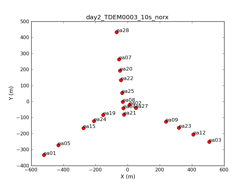
Next, look at a graphical plot of the antenna locations and save a hard copy in case you want it later (see Figure 3). This will be useful for picking a reference antenna—typically a good choice is an antenna close to the center of the array. Unless it shows problems after inspection of the data, we provisionally choose ea02.
# In CASA
plotants(vis='day2_TDEM0003_10s_norx',figfile='ant_locations.png')
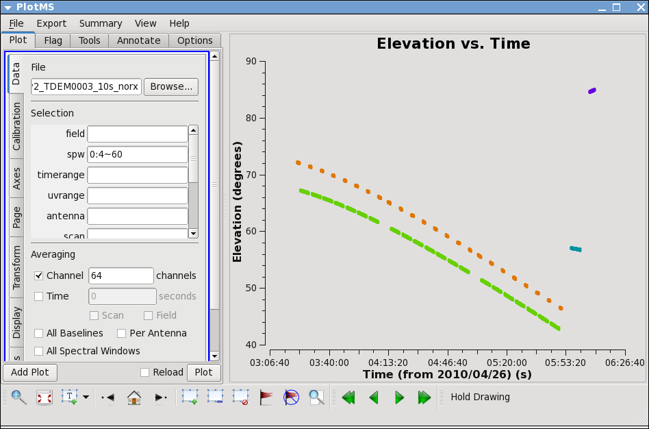
Now look at the elevation as a function of time for all sources (see Figure 4). While it's not the case for these data, you may want to flag if the elevation is very low (usually at the start or end of an observation). Also, how near in elevation your flux calibrator is to your target will impact your ultimate absolute flux density calibration accuracy.
Unfortunately, the target and flux density calibrator are not particularly well-matched for this observation, as you can see by plotting the elevation for each source (each source has a different color). We will be using data in spw 0, channels 4 to 60 for this plot as given by the parameter spw = '0:4~60' ; the general CASA selection syntax is described in the Measurement Selection Syntax Document. Note that because we have set the channel averaging parameter to 64, but only select 57 channels (4 to 60), CASA will issue a warning about this in the terminal. However, as the extra channels are not selected to contain additional data, this is nothing to be concerned about:
# In CASA
plotms(vis='day2_TDEM0003_10s_norx',
       xaxis='time',yaxis='elevation',correlation='RR,LL',
       avgchannel='64',spw='0:4~60', coloraxis='field')
Thus, we are strongly dependent on the opacity and gaincurve corrections to get the flux scale right for these data. (This is something to keep in mind when planning observations.) We will deal with this after the initial inspection.
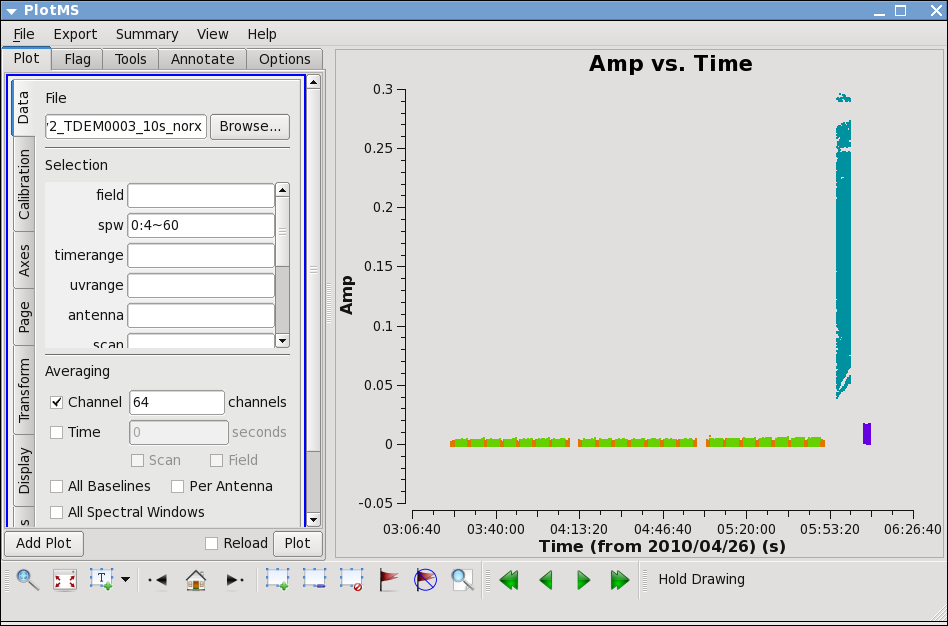
Next, look at all the source amplitudes as a function of time (see Figure 5):
# In CASA
plotms(vis='day2_TDEM0003_10s_norx',
       xaxis='time',yaxis='amp',correlation='RR,LL',
       avgchannel='64',spw='0:4~60', coloraxis='field')
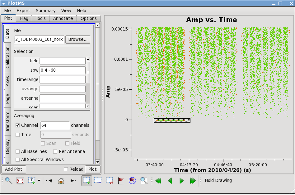
Now zoom in on the region very near zero amplitude for sources J0954+1743 and IRC+10216 (see Figure 6). To zoom, select the
Zoom tool ![]() in the lower left corner of the plotms GUI, then you can left click to draw a box.
Look for the low values (you may want to zoom in a few times to really see the suspect points clearly). Now use the Mark Region
in the lower left corner of the plotms GUI, then you can left click to draw a box.
Look for the low values (you may want to zoom in a few times to really see the suspect points clearly). Now use the Mark Region ![]() and Locate
and Locate ![]() buttons (positioned along the bottom of the GUI) to see which antenna is causing problems. The output is be shown in the logger. Since all the located baselines include ea12, this is the responsible antenna.
buttons (positioned along the bottom of the GUI) to see which antenna is causing problems. The output is be shown in the logger. Since all the located baselines include ea12, this is the responsible antenna.
IMPORTANT NOTES ON PLOTMS:

* When using the locate button, it is important to have only selected a modest number
of points with the mark region tool (see example of marked region in the thumbnail),
otherwise the response will be very slow and possibly hang the tool
(all of the information will be output to your terminal window, not the logger).

* Throughout the tutorial, when you are done marking/locate, use the Clear Regions
tool to get rid of the marked box before plotting other things.

* After flagdata command flagging, you have to force a complete reload of the cache
to look at the same plot again with the new flags applied. To do this, either check
the "force reload" box in the lower left, or do Shift+Plot.

* Fields in the plotms GUI tabs can be altered and the data replotted
without having to close and restart plotms. After you make the changes, click the
Reload box and then click the Plot button adjacent to the Reload box.
Now click the clear region ![]() button, then go back to the zoom button to zoom in further to note exactly what the time range is: 03:41:00~04:10:00.
button, then go back to the zoom button to zoom in further to note exactly what the time range is: 03:41:00~04:10:00.
Check the other sideband by changing spw to 1:4~60. You will have to re-zoom. If you have trouble, click on the Mark icon and then back to zoom. In spw 1, ea07 is bad from the beginning until after the next pointing run: within the Data tab of plotms, set the timerange parameter to 03:21:40~04:10:00. To see this, compare the amplitudes when antenna is set to 'ea07' and when it is set to one of the other antennas, such as 'ea08'.
If you set antenna to 'ea12' and zoom in on this initial time range, you can also see that ea12 is bad during the same time range as for spw 0. You can also see this by entering '!ea07' in the antenna parameter, which removes ea07 from the plot (in CASA, ! deselects).
We can set up a flagging command to get both bad antennas for the appropriate time and spw:
# In CASA
flagdata(vis='day2_TDEM0003_10s_norx',
         mode='list',
         inpfile=["field='2,3' antenna='ea12' timerange='03:41:00~04:10:00'",
                  "field='2,3' antenna='ea07' timerange='03:21:40~04:10:00' spw='1'"])
Task flagdata in mode='list' can take several commands separated by commas. The data selection will be connected by AND for each string.
Note that because the chosen time range is limited to fields 2 and 3, the field parameter is not really needed but the above is a nice example of the task syntax.
Now remove the !ea07 from the antenna parameter and replot both spw, zooming in to be sure that all obviously low points are gone. Also zoom in and check 3C286 (J1229+0203 is already obvious because it is so bright!).
Next, look more closely at IRC+10216:
# In CASA
plotms(vis='day2_TDEM0003_10s_norx',field='3',
       xaxis='time',yaxis='amp',correlation='RR,LL',
       avgchannel='64',spw='0~1:4~60', coloraxis='spw')
You can see that there are some noisy high points. So now try:
# In CASA
plotms(vis='day2_TDEM0003_10s_norx',field='3',
       xaxis='uvdist',yaxis='amp',correlation='RR,LL',
       avgchannel='64',spw='0~1:4~60', coloraxis='spw')
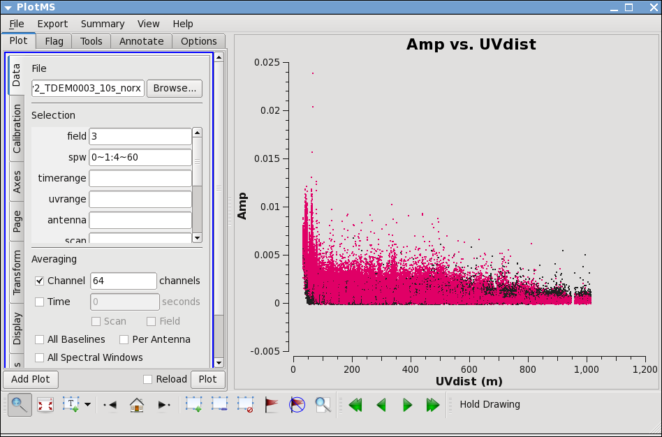
Now we can see that most of the high points on IRC+10216 are due to large scale emission on short baselines (see Figure 7), but there is still some noisy stuff—for a target like this with extended emission it's best to wait until later to decide what to do about it. We will not be able to get adequate calibration for antennas that are truly bad (even if they don't stand out here), so these will be obvious later.
The Observing Log, Antenna Position Corrections, Opacities, Gaincurves, Antenna Efficiencies and other Calibration "Priors"
Antenna Position Corrections
As mentioned in the observing log above, antennas ea10, ea12, and ea22 do not have good baseline positions. Antenna ea10 was not in the array, but for the other two antennas we need to check for any improved baseline positions that were derived after the observations were taken. In CASA, these corrections can be derived by gencal for the JVLA. The parameter caltype='antpos' will use antenna position offset values and create a calibration table for the delay changes that this correction involves. If the 'antenna' parameter is not specified, gencal will query the Jansky VLA webpages for the offsets (Jansky VLA/VLA Baseline Corrections page).
# In CASA
gencal(vis='day2_TDEM0003_10s_norx',caltable='antpos.cal',
       caltype='antpos',
       antenna='')
which return the antenna offsets in the logger:
Determine antenna position offests from the baseline correction database
offsets for antenna ea01 :  0.00000   0.00300   0.00000
offsets for antenna ea02 : -0.00080   0.00000   0.00000
offsets for antenna ea03 : -0.00280   0.00000   0.00000
offsets for antenna ea05 :  0.00000   0.00280   0.00000
offsets for antenna ea12 : -0.01000   0.00450  -0.00170
offsets for antenna ea22 : -0.02570   0.00270  -0.01900
offsets for antenna ea23 : -0.00140   0.00000   0.00000
offsets for antenna ea24 : -0.00150   0.00000   0.00000
offsets for antenna ea27 :  0.00000   0.00190  -0.00160
Please note: if you are reducing VLA data taken before March 1, 2010, you need to set caltype='antposvla' . For the VLA before the conversion to the Jansky VLA, the automated lookup will not work and one has to specify the the antenna positions explicitly.
Gaincurves and Antenna Efficiencies
The gaincurve describes how each antenna behaves as a function of elevation, for each receiver band. Currently, only gaincurves for the VLA are available. This option should not be used with any other telescopes.
Gaincurves are generated into a separate calibration table using the task gencal with the caltype='gceff' . This option will also include antenna efficiencies in the resulting calibration table:
# In CASA
gencal(vis='day2_TDEM0003_10s_norx',caltable='gaincurve.cal',
       caltype='gceff')
Opacities
The opacity of the observation can be computed from a seasonal model and/or weather station information. We are planning to have a task available for this information. At the moment, the CASA_EVLA_Scripts page hosts a script and a contributed task to display the weather information and to calculate the zenith opacities for each spectral window. After the zenith opacities are derived, they will be recomputed for the correct elevation of the data automatically using [math]\displaystyle{ e^{(-\csc[el]\tau_z)} }[/math] in gaincal, applycal, bandpass, etc.
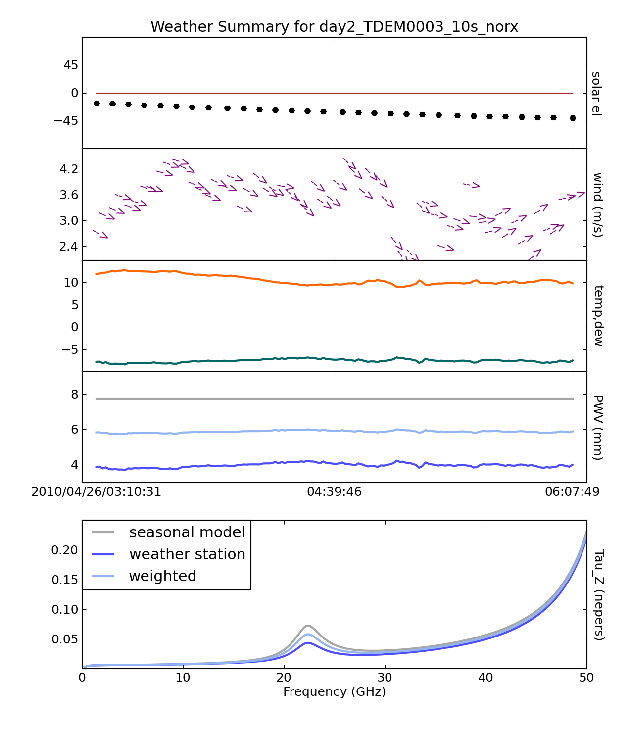
To start, we want to plot the opacity of the atmosphere at 36 GHz at the time this observation was taken so it can be corrected for in subsequent calibrations. The task plotweather takes care of that. The task plots the weather conditions at the time of the observations and calculate the atmospheric opacities based on these data in combination with a seasonal model that contains long-term statistics at the VLA site (see Figure 8). The parameter 'seasonal_weight=0.5' gives both equal weights:
We will be running plotweather in a way that will assign the opacity list (one entry for each spw in ascending order) to the variable myTau:
# In CASA
myTau = plotweather(vis='day2_TDEM0003_10s_norx', doPlot=T)
With this input, the task
- returns the opacity values to the logger:
SPW : Frequency (GHz) : Zenith opacity (nepers)
 0  :   36.387  :  0.039
 1  :   36.305  :  0.039
wrote weather figure: day2_TDEM0003_10s_norx.plotweather.png
- creates a file "day2_TDEM0003_10s_norx.plotweather.png" (in the current working directory) with the elevation of the sun, wind speed and direction, temperature, and precipitable water vapor (PWV) as functions of time over the observation. View this file with your preferred image viewer like gthumb, xv, or Preview;
- and assigns the myTau variable to the list of opacities per spectral window:
# In CASA
myTau
[0.039229977911770554, 0.038993893363737792]
We can now create a calibration table for the opacities via gencal with the calmode='opac' parameter; we can either input the opacities directly or use the myTau variable:
# In CASA
gencal(vis='day2_TDEM0003_10s_norx',caltable='opacity.cal',
       caltype='opac',
       spw='0,1',
       parameter=myTau)
Set Up the Model for the Flux Calibrator
Next, we set the model for the flux calibrator. Depending on your observing frequency and angular resolution you can do this several ways. In the past, one typically used a point source (constant flux) model for the flux calibrator, possibly with a uvrange cutoff if necessary. More recently, model images for the most common flux calibrators have been made available for use in cases where the sources are somewhat resolved. This is most likely to be true at higher frequencies and at higher resolutions (more extended arrays).
The VLA flux calibrator models that are available in CASA can be checked through setjy:
# In CASA
setjy(vis='day2_TDEM0003_10s_norx',listmodels=T)
The terminal will now show the models, e.g., 3C286_C.im, 3C48_K.im, etc. Task setjy will search in the current working directory for images that may contain models, as well as in a CASA directory where known calibrator models are stored.
We will pick the Ka ('A') band model of 3C286: 3C286_A.im. Task setjy scales the total flux in the model image to that appropriate for your individual spectral window frequencies according to the calibrator's flux and reports this number to the logger—it is a good idea to save this information for your records.
# In CASA
setjy(vis='day2_TDEM0003_10s_norx',field='7',spw='0~1',
      scalebychan=T,
      model='3C286_A.im')
The logger output for each spw is:
J1331+3030 (fld ind 7) spw 0  [I=1.7483, Q=0, U=0, V=0] Jy @ 3.6387e+10Hz, (Perley-Butler 2013)
J1331+3030 (fld ind 7) spw 1  [I=1.7512, Q=0, U=0, V=0] Jy @ 3.6305e+10Hz, (Perley-Butler 2013)
Using model image /home/casa/packages/RHEL6/release/casa-release-4.5.0-el6/data/nrao/VLA/CalModels/3C286_A.im
Scaling spw(s) [0, 1]'s model image by channel to  I = 1.75124, 1.7496, 1.74797 Jy @(3.63045e+10, 3.63499e+10, 3.63951e+10)Hz (LSRK) for visibility prediction (a few representative values are shown).
The absolute fluxes for the frequencies of all channels have now been determined, and one can proceed to the bandpass and complex gain calibrations.
Bandpass and Delay
Before determining the bandpass solution, we need to inspect phase and amplitude variations with time and frequency on the bandpass calibrator to decide how best to proceed. We limit the number of antennas to make the plot easier to see. We chose ea02 as it seems like a good candidate for the reference antenna.
# In CASA
plotms(vis='day2_TDEM0003_10s_norx',field='5',
       xaxis='channel',yaxis='phase',correlation='RR',
       avgtime='1e8',spw='0:4~60',antenna='ea02&ea23')
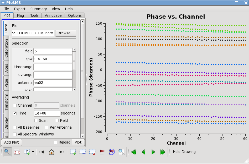
The phase variation is modest ~10 degrees (see Figure 9). Now expand to all baselines that include ea02, and add an extra dimension of color:
# In CASA
plotms(vis='day2_TDEM0003_10s_norx',field='5',
       xaxis='channel',yaxis='phase',correlation='RR',
       avgtime='1e8',spw='0:4~60',antenna='ea02', coloraxis='antenna2')
From this you can see that the phase variation across the bandpass is modest. Next check LL, and then spw=1 for both correlations. Also check other antennas if you like.
Now look at the phase as a function of time:
# In CASA
plotms(vis='day2_TDEM0003_10s_norx',field='5',
       xaxis='time',yaxis='phase',correlation='RR',
       avgchannel='64',spw='0:4~60',antenna='ea02&ea23')
Expand to all antennas with ea02:
# In CASA
plotms(vis='day2_TDEM0003_10s_norx',field='5',
       xaxis='time',yaxis='phase',correlation='RR',
       avgchannel='64',spw='0:4~60',antenna='ea02', coloraxis='antenna2')
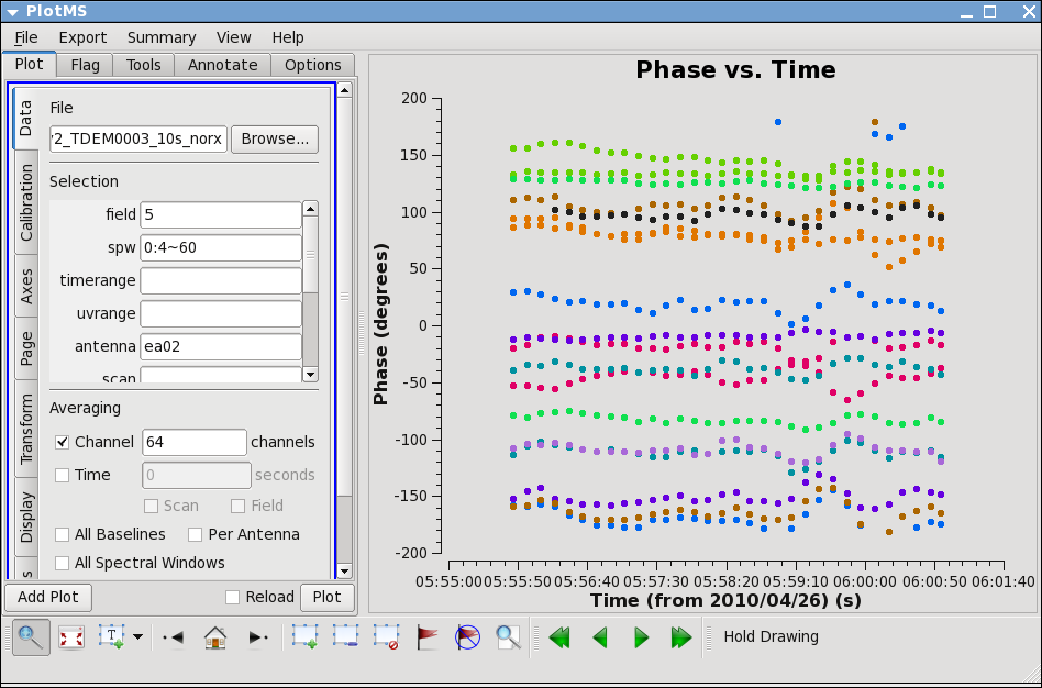
You can see that the phase variations are smooth (see Figure 10), but do vary significantly over the 5 minutes of observation—in most cases by a few 10s of degrees. If you want, zoom in to see this better.
The conclusion from this investigation is that you need to correct the phase variations with time before solving for the bandpass to prevent decorrelation of the vector averaged bandpass solution. Since the phase variation as a function of channel is modest, you can average over several channels to increase the signal to noise of the phase vs. time solution. If the phase variation, as a function of channel is larger, you may need to use only a few channels to prevent introducing delay-based closure errors as can happen from averaging over non-bandpass corrected channels with large phase variations.
Let's take care of the delay calibration first. The delay is the slope of phase across frequency. From the plot we saw that it was rather modest and the bandpass calibration will certainly take care of it. Nevertheless, it might be good to derive a delay calibration first and then calculate the bandpass. The delay calibration is an antenna based calibration solution and it can be derived in gaincal with parameter gaintype='K' .
# In CASA
gaincal(vis='day2_TDEM0003_10s_norx', caltable='delays.cal', field='5',
        refant='ea02', gaintype='K', gaintable=['antpos.cal','gaincurve.cal','opacity.cal'])
We use the strong bandpass calibrator for the solution. It will be extrapolated in time to all observations.
This call also exemplifies how the CASA calibration table system works. Calibration tables are incremental. So we supply the previous 'antpos.cal', 'gaincurve.cal', and 'opacity.cal' tables as input to gaincal. The following calibration step will require the parameter gaintable=['antpos.cal','gaincurve.cal','opacity.cal','delay.cal'] and so on.
Now we proceed to the actual bandpass calibration.
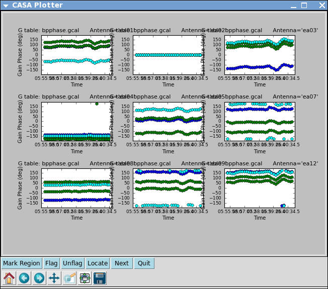
Since the bandpass calibrator is quite strong we do the phase-only
solution on the integration time of 10 seconds (parameter solint='int' ).
# In CASA
gaincal(vis='day2_TDEM0003_10s_norx',caltable='bpphase.gcal',
        field='5',spw='0~1:20~40',
        refant='ea02',calmode='p',solint='int',minsnr=2.0,
        gaintable=['antpos.cal','gaincurve.cal','opacity.cal','delays.cal'])
Plot the solutions (see Figure 11) (note that plotms can also be used for plotting calibration tables):
# In CASA
plotcal(caltable='bpphase.gcal',xaxis='time',yaxis='phase',
        iteration='antenna',subplot=331,plotrange=[0,0,-180,180])
These solutions will appear in the CASA plotter GUI. If you closed it after plotting the antennas positions above, it should reopen. If it is still open from before, the new plots should just appear. After you are done looking at the first set of plots, push the Next button on the GUI to see the next set of antennas.
Now we can apply this phase solution on-the-fly while determining the bandpass solutions on the timescale of the bandpass calibrator scan (parameter solint='inf' ).
We also use the opacity list now instead of myTau—but both options will work.
# In CASA
bandpass(vis='day2_TDEM0003_10s_norx',caltable='bandpass.bcal',field='5',
        refant='ea02',solint='inf',solnorm=T,
        gaintable=['antpos.cal','gaincurve.cal','opacity.cal','delays.cal','bpphase.gcal'])
A few words about solint and combine:
The use of parameter solint='inf' in bandpass will derive one bandpass solution for the whole J1229+0203 scan. Note that if there had been two observations of the bandpass calibrator, this command would have combined the data from both scans to form one bandpass solution, because the default of the combine parameter for bandpass is combine='scan' . To solve for one bandpass for each bandpass calibrator scan you would also need to include combine=' ' in the bandpass call. In all calibration tasks, regardless of solint, scan boundaries are only crossed when combine='scan' . Likewise, field (spw) boundaries are only crossed if parameter combine='field' or parameter combine='spw' , the latter two are not generally good ideas for bandpass solutions.
Plot the solutions, amplitude (see Figure 12) and phase (see Figure 13):
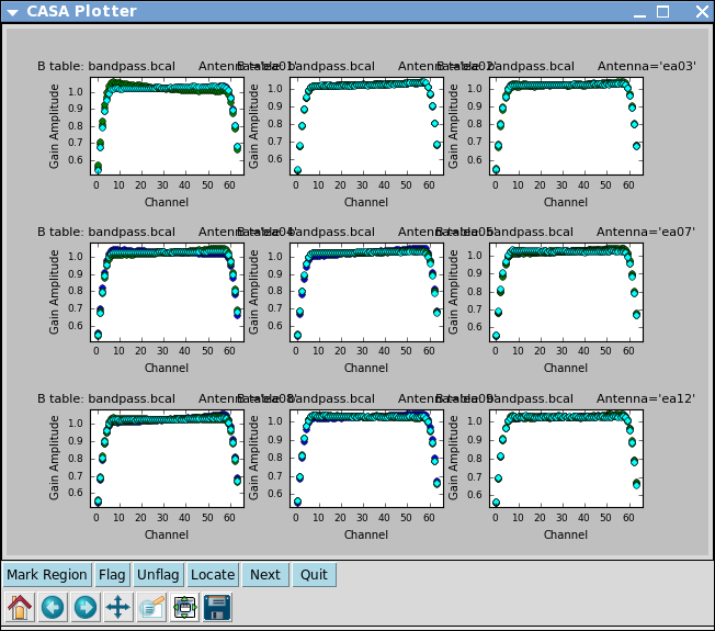
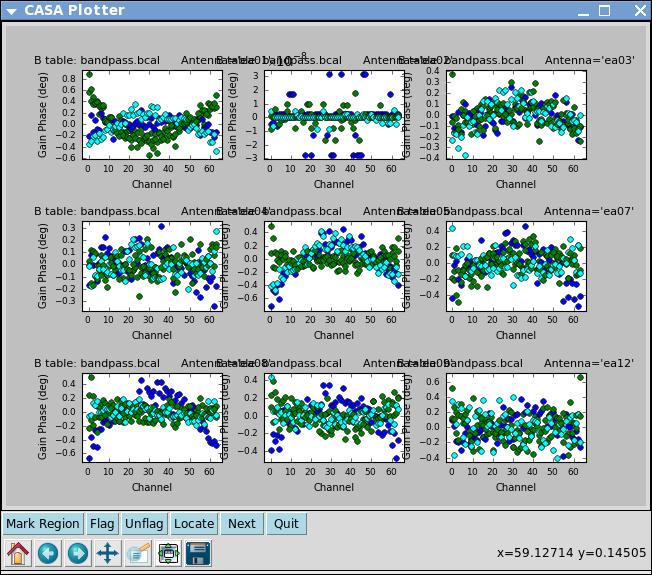
# In CASA
plotcal(caltable='bandpass.bcal',xaxis='chan',yaxis='amp',
        iteration='antenna',subplot=331)
# In CASA
plotcal(caltable='bandpass.bcal',xaxis='chan',yaxis='phase',
        iteration='antenna',subplot=331)
Note the scale for the phases, they are very small since the delays were already taken out in a previous setup.
This step isn't necessary from a calibration perspective, but if you want to go ahead and check the bandpass calibration on the bandpass calibrator you can run applycal here. In the future we hope to plot corrected data on-the-fly without this applycal step. Subsequent applycals will overwrite this one, so no need to worry.
applycal(vis='day2_TDEM0003_10s_norx',field='5',
        gaintable=['antpos.cal','gaincurve.cal','opacity.cal','delays.cal','bandpass.bcal'],
        gainfield=['','','','5','5'],
        calwt=F)
Task applycal works like a matrix. The first entries in the lists are to be used together, so are the second entries etc. (except for the opacity list, which is referring to spws). All will be applied to the 'field' selection. In the above example, 'antpos.cal' from any field is applied to source '5', and the 'bandpass.cal' that was obtained for field '5' (the bandpass observation) is also applied to field '5'. Again, lists within the lists are fine.
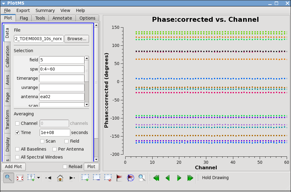
plotms(vis='day2_TDEM0003_10s_norx',field='5',
       xaxis='channel',yaxis='phase',ydatacolumn='corrected',
       correlation='RR',
       avgtime='1e8',spw='0:4~60',antenna='ea02', coloraxis='antenna2')
plotms(vis='day2_TDEM0003_10s_norx',field='5',
       xaxis='channel',yaxis='amp',ydatacolumn='corrected',
       correlation='RR',
       avgtime='1e8',spw='0:4~60',antenna='ea02', coloraxis='antenna2')
Note that the phase and amplitude as a function of channel are very flat now (see Figure 14).
Gain Calibration
Now that we have a bandpass solution to apply, we can solve for the antenna-based phase and amplitude gain calibration. Since the phase changes on a much shorter timescale than the amplitude, we will solve for them separately. If the phase changes significantly over a scan time and if the un-corrected phase were averaged over this timescale, the amplitude would become decorrelated. Note that we re-solve for the gain solutions of the bandpass calibrator to derive new solutions that are corrected for the bandpass shape. Since the bandpass calibrator will not be used again, while not strictly necessary, it is useful to check its calibrated flux density. We use a minimum signal-to-noise of 2 here as it seems to be a good compromise for using good data without rejecting too many solutions (parameter minsnr = 2 ).
# In CASA
gaincal(vis='day2_TDEM0003_10s_norx',caltable='intphase.gcal',
        field='2,5,7',spw='0~1:4~60',
        refant='ea02',calmode='p',solint='int',minsnr=2.0,
        gaintable=['antpos.cal','gaincurve.cal','opacity.cal','delays.cal','bandpass.bcal'])
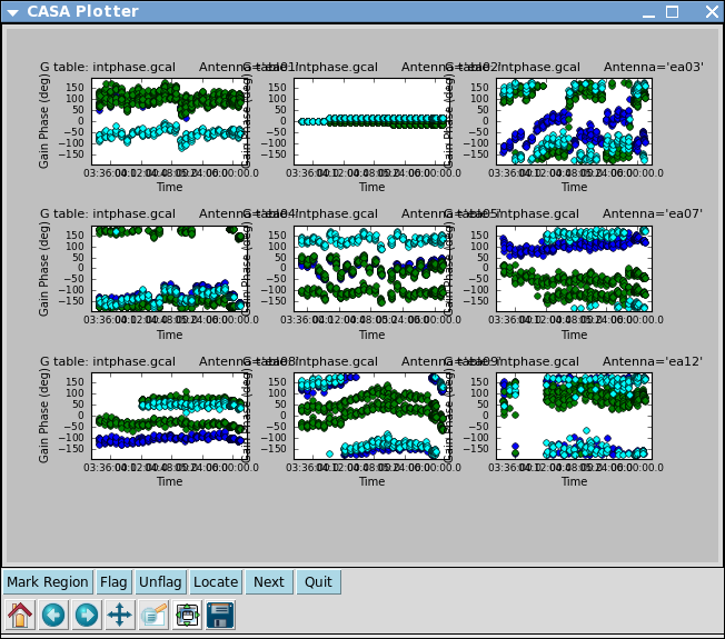
Here parameter solint='int' coupled with parameter calmode='p' will derive a single phase solution for each 10 second integration. Note that the bandpass table is applied on-the-fly before solving for the phase solutions, however the bandpass is NOT applied to the data permanently until applycal is run later on.
Mark that quite a few solutions are rejected due to SNR < 2 (printed to terminal). For the most part it is only one or two solutions out of >30 so this isn't too worrying. Take note if you see large numbers of rejected solutions per integration; this is likely an indication that solint is too short for the S/N of the data.
Now look at the phase solution, and note the obvious scatter within a scan time (see Figure 15):
# In CASA
plotcal(caltable='intphase.gcal',xaxis='time',yaxis='phase',
        iteration='antenna',subplot=331,plotrange=[0,0,-180,180])
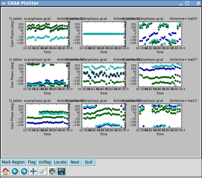
Although solint='int' (i.e. the integration time of 10 seconds) is the best choice to apply before for solving for the amplitude solutions, it is not a good idea to use this to apply to the target. This is because the phase-scatter within a scan can dominate the interpolation between calibrator scans. Instead, we also solve for the phase on the scan time, solint='inf' (but combine=' ' , since we want one solution per scan) for application to the target later on. Unlike the bandpass task, the default of the combine parameter in the gaincal task is combine=' ' .
# In CASA
gaincal(vis='day2_TDEM0003_10s_norx',caltable='scanphase.gcal',
        field='2,5,7',spw='0~1:4~60',
        refant='ea02',calmode='p',solint='inf',minsnr=2.0,
        gaintable=['antpos.cal','gaincurve.cal','opacity.cal','delays.cal','bandpass.bcal'])
# In CASA
plotcal(caltable='scanphase.gcal',xaxis='time',yaxis='phase',
        iteration='antenna',subplot=331,plotrange=[0,0,-180,180])
Note that there are no failed solutions here because of the added S/N afforded by the longer solint (see Figure 16). Alternatively, instead of making a separate phase solution for application to the target, one can also run smoothcal to smooth the solutions derived on the integration time.
Next we apply the bandpass and parameter solint='int' phase-only calibration solutions on-the-fly to derive amplitude solutions. Here the use of solint='inf' , not combine=' ' ,will result in one solution per scan interval.
# In CASA
gaincal(vis='day2_TDEM0003_10s_norx',caltable='amp.gcal',
        field='2,5,7',spw='0~1:4~60',
        refant='ea02',calmode='ap',solint='inf',minsnr=2.0,
        gaintable=['antpos.cal','gaincurve.cal','opacity.cal','delays.cal','bandpass.bcal','intphase.gcal'])
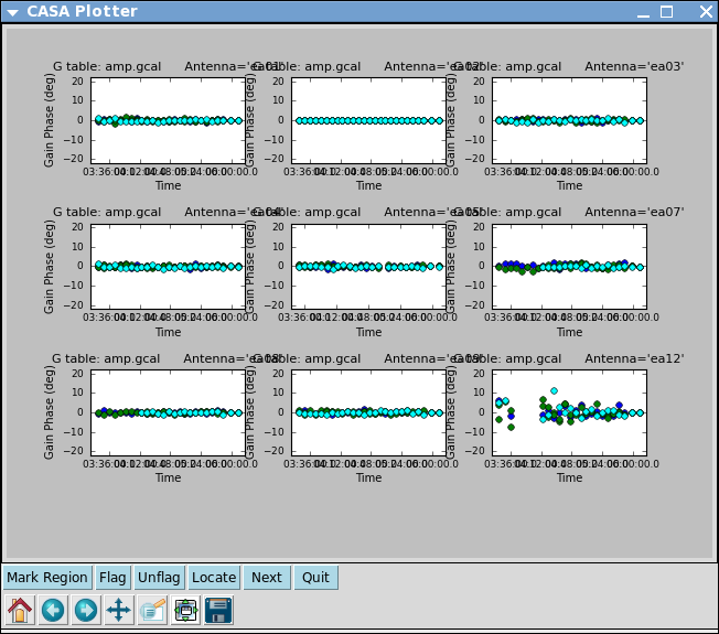
Now let's look at the resulting phase solutions (see Figure 17). Since we have taken out the phase as best we can by applying the solint='int' phase-only solution, this plot will give a good idea of the residual phase error. If you see scatter of more than a few degrees here, you should consider going back and looking for more data to flag, particularly bad timeranges, etc.
# In CASA
plotcal(caltable='amp.gcal',xaxis='time',yaxis='phase',
        iteration='antenna',subplot=331,plotrange=[-1,-1,-20,20])
Note that we have restricted the plot range so that all antennas are plotted with the same scale (instead of autoscaled; the -1,-1 values for the X-axis allow autoscaling to take place still) (see Figure 18). We can see that both antenna ea12 (all times) and ea23 (first 1/3 of observation) show particularly large residual phase noise.
# In CASA
plotcal(caltable='amp.gcal',xaxis='time',yaxis='amp',
        iteration='antenna',subplot=331,plotrange=[-1,-1,0,1])
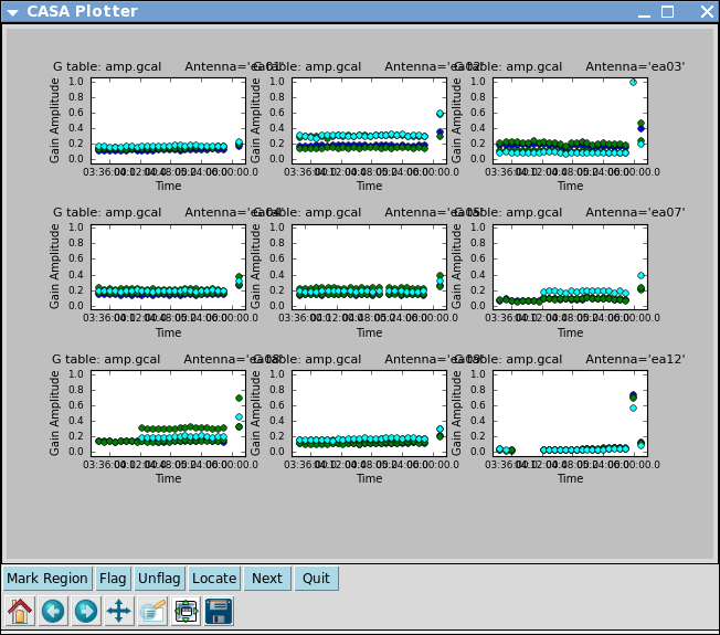
Note that the amplitude solutions for ea12 are very low, in particular when you set plotrange=[-1,-1,0,1]; this is another indication that this antenna is dubious.
Next we use the flux calibrator (whose flux density was set in setjy above) to derive the flux of the other calibrators (see Figure 19). Note as of CASA 4.0, the flux table can be written as an incremental table, just like all other calibration tables. In that case it won't replace the amp.gcal but both tables, amp.gcal as well as flux.gcal need to be carried onward.
# In CASA
fluxscale(vis='day2_TDEM0003_10s_norx',caltable='amp.gcal',
          fluxtable='flux.cal',reference='7',incremental=T)
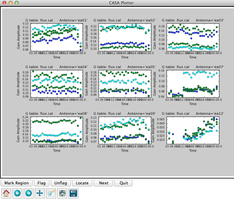
It is a good idea to note down for your records the derived flux densities:
Found reference field(s): J1331+3030
Found transfer field(s):  J0954+1743 J1229+0203

Flux density for J0954+1743 in SpW=0 (freq=3.63912e+10 Hz) is: 0.221057 +/- 0.0307662 (SNR = 7.18507, N = 38)
Flux density for J0954+1743 in SpW=1 (freq=3.63085e+10 Hz) is: 0.227938 +/- 0.0297123 (SNR = 7.67149, N = 38)
Flux density for J1229+0203 in SpW=0 (freq=3.63912e+10 Hz) is: 27.2661 +/- 0.245123 (SNR = 111.235, N = 38)
Flux density for J1229+0203 in SpW=1 (freq=3.63085e+10 Hz) is: 26.554 +/- 0.2568 (SNR = 103.403, N = 38)
Applycal and Inspect
Now we apply the calibration to each source according to which tables are appropriate and which source should be used to do that particular calibration. For the calibrators, all bandpass solutions come from the bandpass calibrator (id=5), and the phase and amplitude calibration comes from their own solutions.
Note: In all applycal steps we set calwt=F. It is very important to turn off this parameter which determines if the weights are calibrated along with the data. Data from antennas with better receiver performance and/or longer integration times should have higher weights, and it can be advantageous to factor this information into the calibration. During the VLA era, meaningful weights were available for each visibility. However, at the time of this observation, the VLA was not yet recording the information necessary to calculate meaningful weights. Since these data weights are used at the imaging stage you can get strange results from having calwt=T when the input weights are themselves not meaningful, especially for self-calibration on resolved sources (for example, flux calibrator and target).
For more recent data, the switched power information is recorded, but we currently do not recommend using this information to calculate data weights without exercising considerable caution.
# In CASA
# for the gain/phase calibrator (field '2'):
applycal(vis='day2_TDEM0003_10s_norx',field='2',
        gaintable=['antpos.cal','gaincurve.cal','opacity.cal','delays.cal','bandpass.bcal','intphase.gcal','amp.gcal','flux.cal'],
        gainfield=['','','','5','5','2','2','2'],
        calwt=F)
# In CASA
# for the bandpass calibrator (field '5'):
applycal(vis='day2_TDEM0003_10s_norx',field='5',
        gaintable=['antpos.cal','gaincurve.cal','opacity.cal','delays.cal','bandpass.bcal','intphase.gcal','amp.gcal','flux.cal'],
        gainfield=['','','','5','5','5','5','5'],
        calwt=F)
# In CASA
# for the flux calibrator (field '7'):
applycal(vis='day2_TDEM0003_10s_norx',field='7',
        gaintable=['antpos.cal','gaincurve.cal','opacity.cal','delays.cal','bandpass.bcal','intphase.gcal','amp.gcal','flux.cal'],
        gainfield=['','','','5','5','7','7','7'],
        calwt=F)
For the target we apply the bandpass (id=5), and the calibration from the gain calibrator (id=2):
# In CASA
# for the target source IRC10216 (field '3'):
applycal(vis='day2_TDEM0003_10s_norx',field='3',
        gaintable=['antpos.cal','gaincurve.cal','opacity.cal','delays.cal','bandpass.bcal','scanphase.gcal','amp.gcal','flux.cal'],
        gainfield=['','','','5','5','2','2','2'],
        calwt=F)
Now inspect the corrected data:
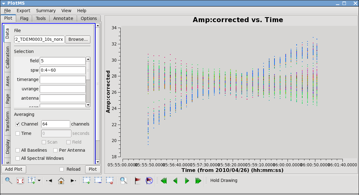
# In CASA
plotms(vis='day2_TDEM0003_10s_norx',field='5',ydatacolumn='corrected',
       xaxis='time',yaxis='amp',correlation='RR,LL',
       avgchannel='64',spw='0:4~60',antenna='', coloraxis='antenna1')
This plot shows some data deviating from the average amplitudes (see Figure 20). Use methods previously described to mark a region for a small number of deviant data points and click Locate. You will find that ea12 is responsible.
# In CASA
plotms(vis='day2_TDEM0003_10s_norx',field='2',ydatacolumn='corrected',
       xaxis='time',yaxis='amp',correlation='RR,LL',
       avgchannel='64',spw='0:4~60',antenna='', coloraxis='antenna2')
Here we see some problems, with high points. Mark some regions and locate in plotms to find out which antennas and in which spws. Pay special attention to antennas that have been called out already as showing some dubious behavior.
What you find is that ea07, which we flagged spw=1 above, is also bad for the same timerange in spw=0. This was not obvious in the raw data because spw=0 was adjusted in the on-line system by a gain attenuator, while spw=1 wasn't. So a lack of power on this antenna can look like very low (and obvious) amplitudes in spw=1 but not for spw=0. Looking carefully you'll see that ea07 is actually pretty noisy throughout.
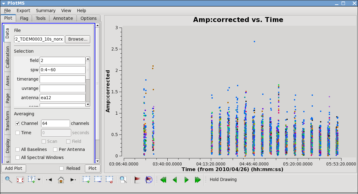
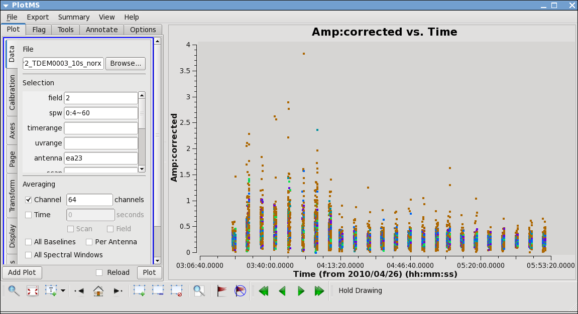
From the locate we also find that ea12 and ea23 show some high points; to see this, replot baselines using each of them alone (see Figures 21 and 22):
plotms(vis='day2_TDEM0003_10s_norx',field='2',ydatacolumn='corrected',
       xaxis='time',yaxis='amp',correlation='RR,LL',
       avgchannel='64',spw='0:4~60',antenna='ea12', coloraxis='antenna2')
plotms(vis='day2_TDEM0003_10s_norx',field='2',ydatacolumn='corrected',
       xaxis='time',yaxis='amp',correlation='RR,LL',
       avgchannel='64',spw='0:4~60',antenna='ea23', coloraxis='antenna2')
It may be a good idea to flag ea12 completely—it's just a bit noisy all around and ea23 is pretty noisy during the first scans between the initial and second pointing. Recall that these are antennas we became suspicious of while inspecting the calibration solutions.
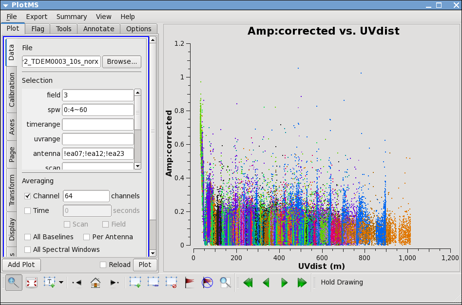
Now let's see how the target looks. Because the target has resolved structure, its best to look at it as a function of uvdistance. We'll go ahead and exclude the three antennas we already know have problems.
# In CASA
plotms(vis='day2_TDEM0003_10s_norx',field='3',ydatacolumn='corrected',
       xaxis='uvdist',yaxis='amp',correlation='RR,LL',
       avgchannel='64',spw='0:4~60',antenna='!ea07;!ea12;!ea23', coloraxis='antenna2')
The color indicates that the spikes are caused by a single antenna (see Figure 23). Use zoom, mark, and locate to see which one. Also look at spw=1.
The bad antenna turns out to be ea28; to confirm, replot with antenna=!ea28:
# In CASA
plotms(vis='day2_TDEM0003_10s_norx',field='3',ydatacolumn='corrected',
       xaxis='uvdist',yaxis='amp',correlation='RR,LL',
       avgchannel='64',spw='0:4~60',antenna='!ea07;!ea12;!ea23;!ea28', coloraxis='antenna2')
Looks much better. To see if it's restricted to a certain time, do:
# In CASA
plotms(vis='day2_TDEM0003_10s_norx',field='3',ydatacolumn='corrected',
       xaxis='time',yaxis='amp',correlation='RR,LL',
       avgchannel='64',spw='0:4~60',antenna='ea28', coloraxis='antenna1')
Baselines with ea28 clearly show issues until about two-thirds of the way through the observation. Plot another distant antenna to compare. We will go ahead and flag it all, since it's hanging far out on the north arm by itself.
The additional data we've identified as bad need to be flagged, and then all the calibration steps will need to be run again.
# In CASA
flagdata(vis='day2_TDEM0003_10s_norx',
         mode='list',
         inpfile=["antenna='ea07,ea12,ea28'",
                   "antenna='ea07,ea23' timerange='03:21:40~04:10:00'"])
Redo Calibration after more Flagging
After flagging, you'll need to repeat the calibration steps above. Here, we append _redo to the table names to distinguish them from the first round, in case we want to compare with previous versions.
# In CASA
gaincal(vis='day2_TDEM0003_10s_norx',caltable='bpphase_redo.gcal',
        field='5',spw='0~1:20~40',
        refant='ea02',calmode='p',solint='int',minsnr=2.0,
        gaintable=['antpos.cal','gaincurve.cal','opacity.cal','delays.cal'])
#
bandpass(vis='day2_TDEM0003_10s_norx',caltable='bandpass_redo.bcal',
        field='5',
        refant='ea02',solint='inf',solnorm=T,
        gaintable=['antpos.cal','gaincurve.cal','opacity.cal','delays.cal','bpphase_redo.gcal'])
#
gaincal(vis='day2_TDEM0003_10s_norx',caltable='intphase_redo.gcal',
        field='2,5,7',spw='0~1:4~60',
        refant='ea02',calmode='p',solint='int',minsnr=2.0,
        gaintable=['antpos.cal','gaincurve.cal','opacity.cal','delays.cal','bandpass_redo.bcal'])
#
gaincal(vis='day2_TDEM0003_10s_norx',caltable='scanphase_redo.gcal',
        field='2,5,7',spw='0~1:4~60',
        refant='ea02',calmode='p',solint='inf',minsnr=2.0,
        gaintable=['antpos.cal','gaincurve.cal','opacity.cal','delays.cal','bandpass_redo.bcal'])
#
gaincal(vis='day2_TDEM0003_10s_norx',caltable='amp_redo.gcal',
        field='2,5,7',spw='0~1:4~60',
        refant='ea02',calmode='ap',solint='inf',minsnr=2.0,
        gaintable=['antpos.cal','gaincurve.cal','opacity.cal','delays.cal','bandpass_redo.bcal','intphase_redo.gcal'])
#
fluxscale(vis='day2_TDEM0003_10s_norx',caltable='amp_redo.gcal',
          fluxtable='flux_redo.cal',reference='7',incremental=T)
Flux density for J0954+1743 in SpW=0 (freq=3.63912e+10 Hz) is: 0.238544 +/- 0.0285193 (SNR = 8.36429, N = 32)
Flux density for J0954+1743 in SpW=1 (freq=3.63085e+10 Hz) is: 0.230267 +/- 0.0291107 (SNR = 7.91006, N = 32)
Flux density for J1229+0203 in SpW=0 (freq=3.63912e+10 Hz) is: 26.3263 +/- 0.285264 (SNR = 92.2876, N = 32)
Flux density for J1229+0203 in SpW=1 (freq=3.63085e+10 Hz) is: 25.7893 +/- 0.292805 (SNR = 88.0769, N = 32)
Feel free to pause here and remake the calibration solution plots from above, just be sure to put in the revised table names.
Redo Applycal and Inspect
Now apply all the new calibrations, which will overwrite the old ones. These commands are identical to those above, with the exception of the _redo part of each calibration filename.
# In CASA
applycal(vis='day2_TDEM0003_10s_norx',field='2',
        gaintable=['antpos.cal','gaincurve.cal','opacity.cal','delays.cal','bandpass_redo.bcal','intphase_redo.gcal','amp_redo.gcal','flux_redo.cal'],
        gainfield=['','','','5','5','2','2','2'],
        calwt=F)
#
applycal(vis='day2_TDEM0003_10s_norx',field='5',
        gaintable=['antpos.cal','gaincurve.cal','opacity.cal','delays.cal','bandpass_redo.bcal','intphase_redo.gcal','amp_redo.gcal','flux_redo.cal'],
        gainfield=['','','','5','5','5','5','5'],
        calwt=F)
#
applycal(vis='day2_TDEM0003_10s_norx',field='7',
        gaintable=['antpos.cal','gaincurve.cal','opacity.cal','delays.cal','bandpass_redo.bcal','intphase_redo.gcal','amp_redo.gcal','flux_redo.cal'],
        gainfield=['','','','5','5','7','7','7'],
        calwt=F)
#
applycal(vis='day2_TDEM0003_10s_norx',field='3',
        gaintable=['antpos.cal','gaincurve.cal','opacity.cal','delays.cal','bandpass_redo.bcal','scanphase_redo.gcal','amp_redo.gcal','flux_redo.cal'],
        gainfield=['','','','5','5','2','2','2'],
        calwt=F)
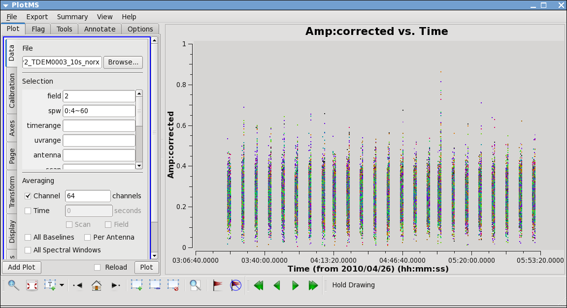
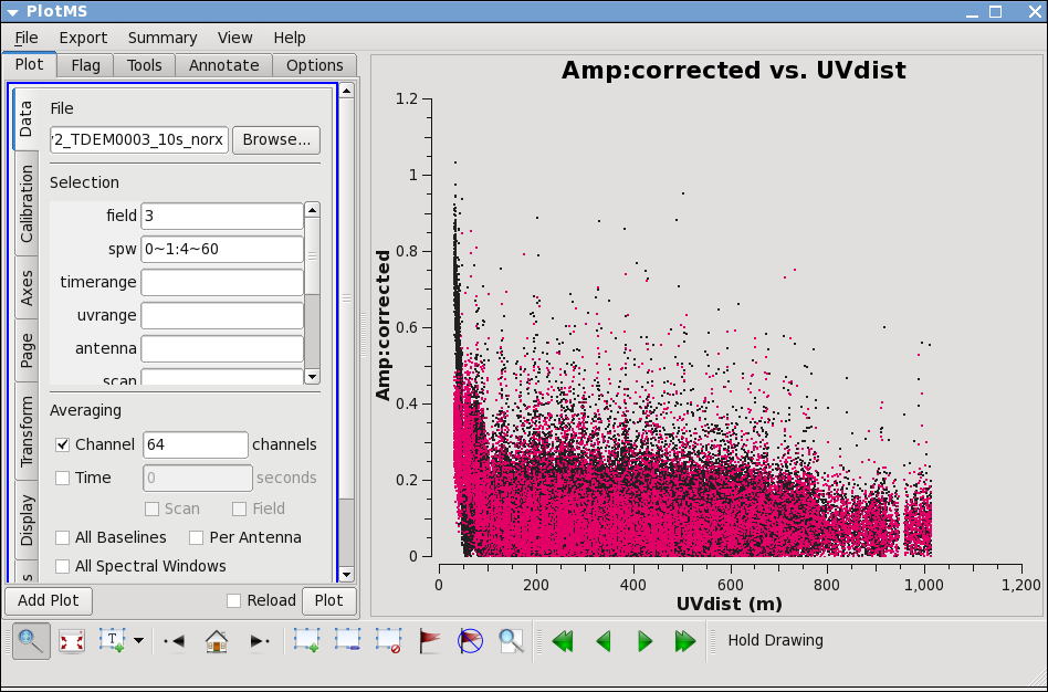
Now you can inspect the calibrated data again (see Figure 24). Except for random scatter, things look pretty good.
# In CASA
plotms(vis='day2_TDEM0003_10s_norx',field='2',ydatacolumn='corrected',
       xaxis='time',yaxis='amp',correlation='RR,LL',
       avgchannel='64',spw='0:4~60',antenna='', coloraxis='antenna2')
You can use the Mark and Locate buttons to assess that the remaining scatter seems random, i.e., no particular antenna or time range appears to be responsible (see Figure 25).
# In CASA
plotms(vis='day2_TDEM0003_10s_norx',field='3',ydatacolumn='corrected',
       xaxis='uvdist',yaxis='amp',correlation='RR,LL',
       avgchannel='64',spw='0~1:4~60',antenna='', coloraxis='spw')
Split
Now we split the data into individual files. This is not strictly necessary, as you can select the appropriate fields in later clean stages, but it is safer in case for example you get confused with later processing and want to fall back to this point (this is especially a good idea if you plan to do continuum subtraction or self calibration later on). It also makes smaller individual files in case you want to copy to another machine or colleague.
Here, we split off the data for the phase calibrator and the target:
# In CASA
split(vis='day2_TDEM0003_10s_norx',outputvis='J0954',
      field='2')
#
split(vis='day2_TDEM0003_10s_norx',outputvis='IRC10216',
      field='3')
This concludes the calibration phase of the data reductions.
UV Continuum Subtraction and Setting Up for Self-Calibration
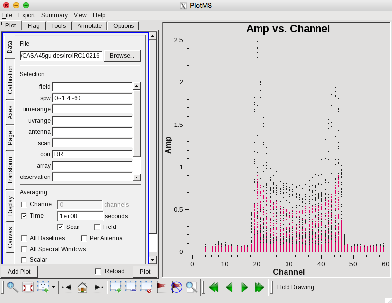
Now we can make a vector averaged uv-plot of the calibrated target spectral line data. It is important to note that you will only see signal in such a plot if (1) the data are well calibrated, and (2) there is significant signal near the phase center of the observations or if the line emission (or absorption) is weak but extended. If this isn't true for your data, you won't be able to see the line signal in such a plot and will need to make an initial (dirty or lightly cleaned) line+continuum cube to determine the line-free channels. Generally, this is the recommended course for finding the line-free channels more precisely than is being done here due to time constraints, as weak line signal would not be obvious in this plot.
plotms(vis='IRC10216',field='',ydatacolumn='data',
       xaxis='channel',yaxis='amp',correlation='RR',
       avgtime='1e8',avgscan=T,spw='0~1:4~60',antenna='', coloraxis='spw')
In the Display tab, change the Unflagged Points Symbol to Custom and Style to circle or diamond and 3 pixels.
You should see the horned profile typical of a rotation shell (see Figure 26). From this plot, you can guess that strong line emission is restricted to channels 18 to 47 (zoom in if necessary to see exactly what the channel numbers are).
In the Data tab, under Averaging, you can also click on All Baselines to average all baselines, but this is a little harder to see.
Now we want to use the line-free channels to create a model of the continuum emission that can be subtracted to form a line-only dataset. We want to refrain from going to close to the edges of the band—these channels are typically noisy, and we don't want to get too close to the line channels because we could only see strong line emission in the vector averaged uv-plot.
We can now either specify the line free channels via parameters fitspw='0~1:4~13;52~63' and excludechans=F in uvcontsub, or do the inverse selection via:
uvcontsub(vis='IRC10216',fitspw='0~1:14~51',excludechans=T,
       want_cont=T)
which excludes the line channels from the continuum fit.
The parameter want_cont=T will produce two new datasets; IRC10216.contsub is the continuum subtracted line data, and IRC10216.cont is the continuum estimate (note however, that it is still a multi-channel dataset).
Velocity Systems and Doppler corrections
The Jansky VLA does not support Doppler tracking. Doppler setting is possible which will calculate the sky frequency based on a velocity of the source at the start of an observation. The sky frequency is then fixed throughout that track. Typically, a fixed frequency is better for the calibration of interferometric data. The downside, however, is that a spectral line may shift over one or more channels during an observation. Task clean takes care of such a shift when regridding the visibilities in velocity space (default is LSRK) to form an image. Sometimes, in particular when adding together different observing tracks, it may be advisable to regrid all data sets to the same velocity grid, combine all data to a single file, then Fourier transform and deconvolve. The tasks cvel, concat, and clean serve this purpose respectively. The following run of cvel shows an example on how the parameters of cvel may be set.
The IRC10216.contsub visibility spans the following channel range (see also the listobs output in the first part of the tutorial):
# In CASA
vishead(vis='IRC10216.contsub', mode='summary')
SpwID  Name      #Chans   Frame   Ch0(MHz)  ChanWid(kHz)  TotBW(kHz) CtrFreq(MHz)  Corrs
0      Subband:0     64   TOPO   36387.229       125.000      8000.0  36391.1670   RR  RL  LR  LL
1      Subband:0     64   TOPO   36304.542       125.000      8000.0  36308.4795   RR  RL  LR  LL
For spw 0, this corresponds to about 1 km/s channel width. If we want to image the HC3N spectral line with a rest frequency of 36.39232 GHz over a velocity range of −50km/s to 0km/s and a channel width of 5 km/s, we may decide to regrid the visibilities in cvel as:
Note that this step is not necessary for the processing further down in this tutorial. You may skip to the next section if you wish.
# In CASA
cvel(vis='IRC10216.contsub', outputvis='IRC10216.contsub-cveled', mode='velocity',
     interpolation='linear', nchan=10, start='-50km/s', width='5km/s',
     restfreq='36.39232GHz',outframe='LSRK', veltype='optical')
This will create a new dataset where the data is binned into the new grid. Since all data in measurement sets are stored in frequency space, an inspection with vishead now gives:
# In CASA
vishead(vis='IRC10216.contsub-cveled', mode='summary')
SpwID  Name      #Chans   Frame   Ch0(MHz)  ChanWid(kHz)  TotBW(kHz) CtrFreq(MHz)  Corrs
0      Subband:0     10   LSRK   36392.927       606.974      6070.6  36395.6588   RR  RL  LR  LL
After the cvel step, the data can then be combined with other observations via concat and imaged in clean with parameter mode='channel' to conserve that velocity system and grid.
Note that cvel can also Hanning smooth the data, if needed (as an alternative to the stand-alone hanningsmooth task).
Image the Spectral Line Data
Here we make images from the continuum-subtracted, calibrated spectral line data. Because the spectral line emission from IRC+10216 has significant extended emission, it is very important to run clean interactively, and make a clean mask. To make the cube a bit smaller and stay away from noisy edge channels we restrict the channel range using the spw parameter.
Note that interrupting clean by Ctrl+C may corrupt your visibilities—you may be better off choosing to let clean finish. We are currently implementing a command that will nicely exit to prevent this from happening, but for the moment try to avoid Ctrl+C.
# In CASA
clean(vis='IRC10216.contsub',imagename='IRC10216_HC3N.cube_r0.5',
      imagermode='csclean',
      imsize=300,cell=['0.4arcsec'],spw='0:5~58',
      mode='velocity',interpolation='linear',
      restfreq='36.39232GHz',outframe='LSRK',
      weighting='briggs',robust=0.5,
      interactive=T,
      threshold='3.0mJy',niter=100000)
- imagermode = csclean will invoke the Cotton-Schwab cleaning algorithm and the data will be regridded into a new output velocity frame, correcting for Doppler shifts of the line during the run (VLA data for each track is always topocentric at a fixed sky frequency). The iterations are chosen as a high value to allow many clean cycles when needed. Typically, however, the threshold will kick in earlier and stop the cleaning process.
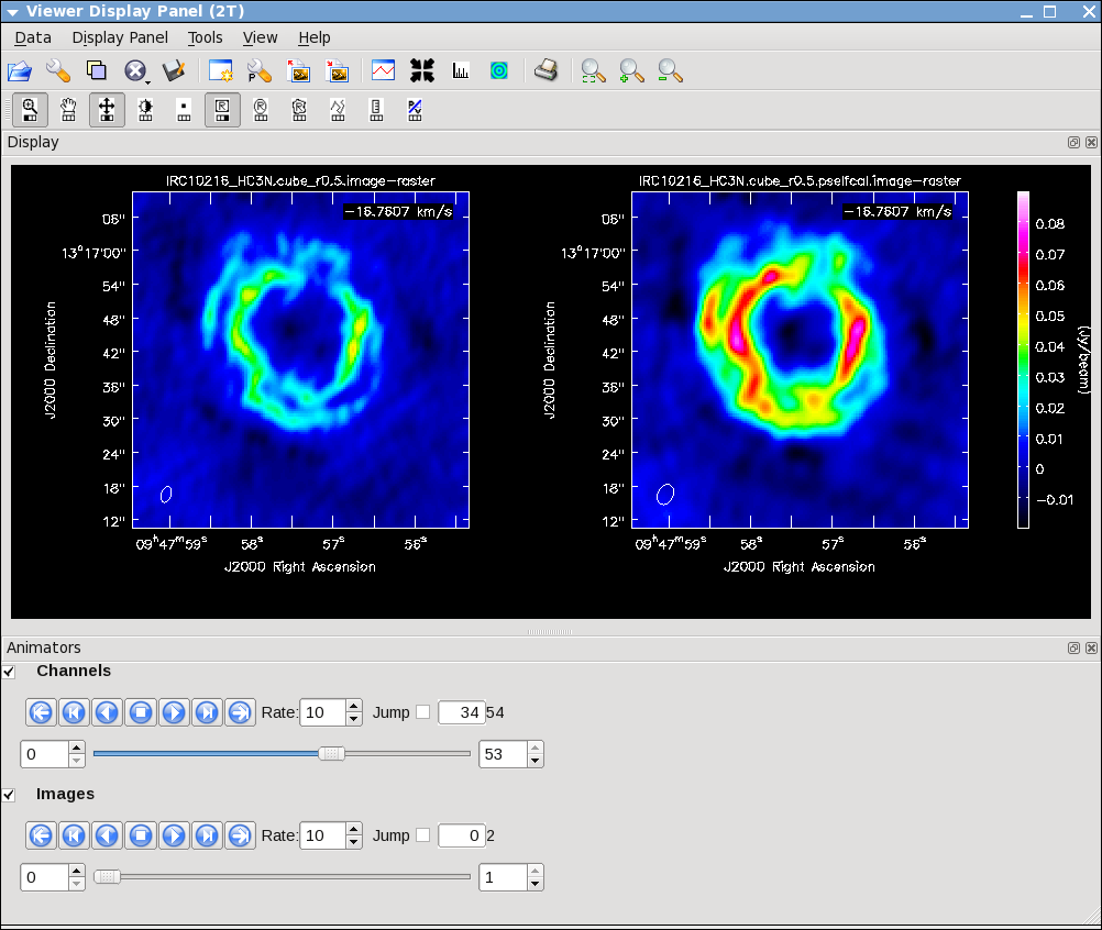
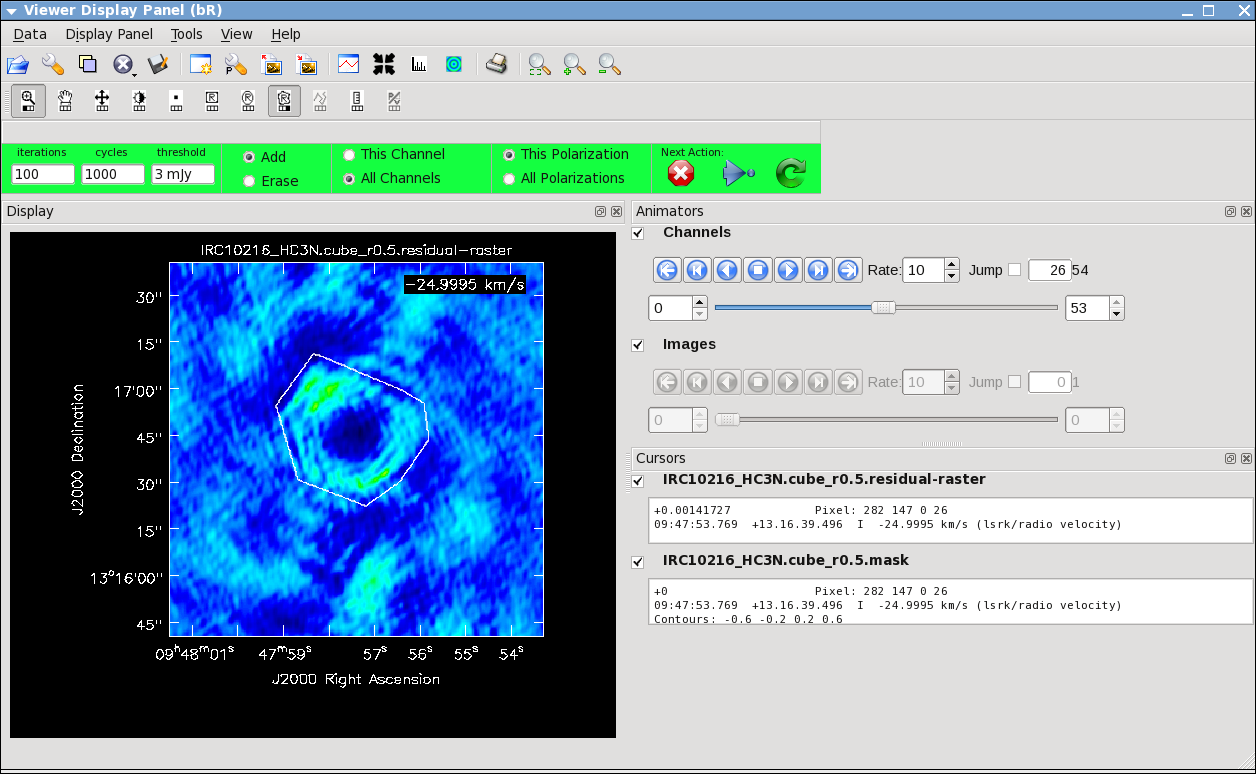
It will take a little while to grid the data, but the viewer will open when it's ready to start an interactive clean. Use the Channels tape deck buttons at the bottom (sometimes it will load on the side) of the Viewer display GUI to step through to the channel with the most extended (in angular size) emission. Select all channels for the clean mask, select the polygon tool ![]() , and make a single mask that applies to all channels by clicking on the image to drop anchor points (see Figure 27) and drawing lines between the points. Once you make the polygon region, you need to double click inside it to save the mask region—if you see the polygon turn white you will know you succeeded. Note, that if you had the time and patience you could make a clean mask for each channel, and this would create a slightly better result.
, and make a single mask that applies to all channels by clicking on the image to drop anchor points (see Figure 27) and drawing lines between the points. Once you make the polygon region, you need to double click inside it to save the mask region—if you see the polygon turn white you will know you succeeded. Note, that if you had the time and patience you could make a clean mask for each channel, and this would create a slightly better result.
After making the mask you should check that the emission in all the other channels fits within the mask you made using the tape deck controls to move back and forth. If you need to include more area in the mask, you can chose the erase toggle at the top, and then encircle your existing mask with a polygon and double click inside. Then go back to add toggle at top and make a new mask. Alternatively, you can erase a part of the mask, or you can add to the existing mask by drawing new polygons. Feel free to experiment with this a bit.
Note: If you start an interactive clean, and then do not make a mask, clean will stop when you tell it to go on because it has nothing to clean. There is no default mask.
To continue with clean use one of the Next action buttons in the green area on the Viewer Display GUI: The red X ![]() will stop clean where you are; the blue arrow
will stop clean where you are; the blue arrow ![]() will stop the interactive part of clean, but continue to clean non-interactively until reaching the stopping niter (iterations x cycles) or threshold—whichever comes first; and the green arrow
will stop the interactive part of clean, but continue to clean non-interactively until reaching the stopping niter (iterations x cycles) or threshold—whichever comes first; and the green arrow ![]() will clean until it reaches the iterations parameter on the left side of the green area. When the interactive viewer comes back use the tape deck to recheck that your mask encompasses what you think is real emission. If your mouse has a middle button, then by default it controls the image stretch.
will clean until it reaches the iterations parameter on the left side of the green area. When the interactive viewer comes back use the tape deck to recheck that your mask encompasses what you think is real emission. If your mouse has a middle button, then by default it controls the image stretch.
For this example, the threshold has been set to threshold = '3mJy' to protect you from cleaning too deeply. With a careful clean mask you can clean too close to the thermal noise limit (the actual observed rms noise limit and not the theoretical one calculated for the proposal, as flagging, weather, etc., can affect what you actually get). It is ALWAYS best to clean each channel in a cube to a specific threshold than to stop by simply using the niter parameter, which can leave each channel cleaned to different levels. There are many ways to determine a suitable threshold. One way is to make a dirty image (niter = 0), open the cube using the viewer, go to a line free channel, select the box region tool, make a box near the field center about the size of your source, and double click inside. The rms noise of that channel will appear in the terminal window from which the viewer was launched. Try a few different boxes and average the results; this is a good estimate of the rms per channel assuming your data are not dynamic range limited (i.e., noise can be higher in channels with strong signal). This is the absolute minimum for threshold and with no mask you probably shouldn't clean deeper than 3x this rms.
Keep cleaning by using the green Next Action arrow ![]() until the residual displayed in the viewer looks noise-like. To speed things up, you might change the iteration parameter in the viewer to something like 300. This parameter can also be set in the task command. You will notice that in this particular case there are residuals that cannot be cleaned—these are due to the extended, resolved out structure on size scales larger than the array is sensitive to (Largest Angular Scale (LAS) that the array is sensitive to can be calculated from the shortest baseline length), and potential residual phase and amplitude calibration errors. We will explore this in a few sections with self-calibration.
until the residual displayed in the viewer looks noise-like. To speed things up, you might change the iteration parameter in the viewer to something like 300. This parameter can also be set in the task command. You will notice that in this particular case there are residuals that cannot be cleaned—these are due to the extended, resolved out structure on size scales larger than the array is sensitive to (Largest Angular Scale (LAS) that the array is sensitive to can be calculated from the shortest baseline length), and potential residual phase and amplitude calibration errors. We will explore this in a few sections with self-calibration.
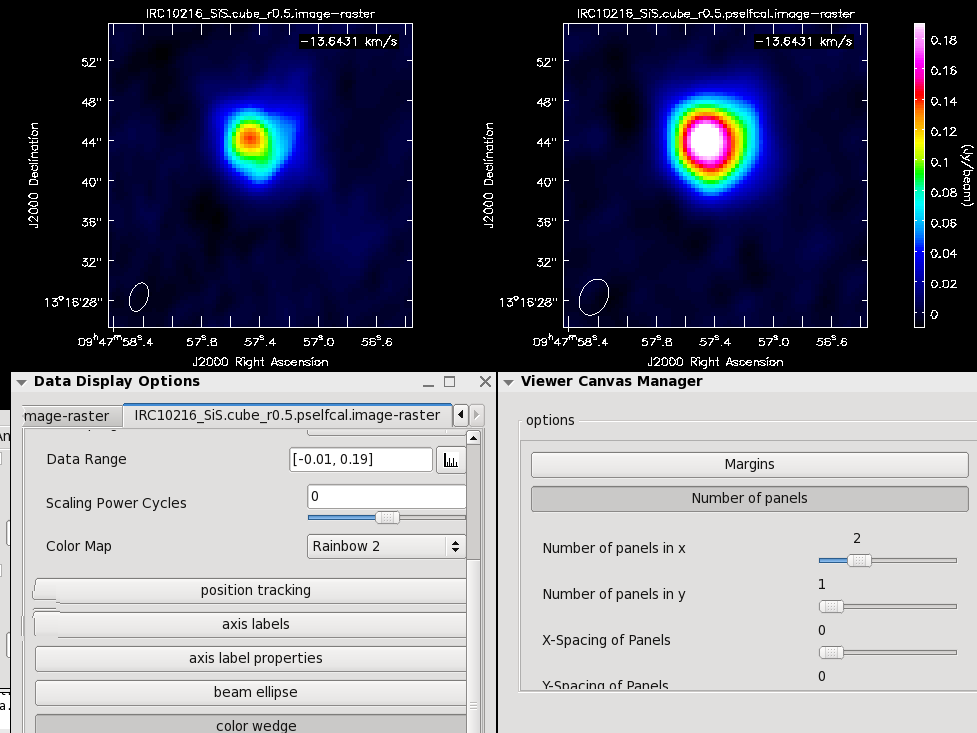
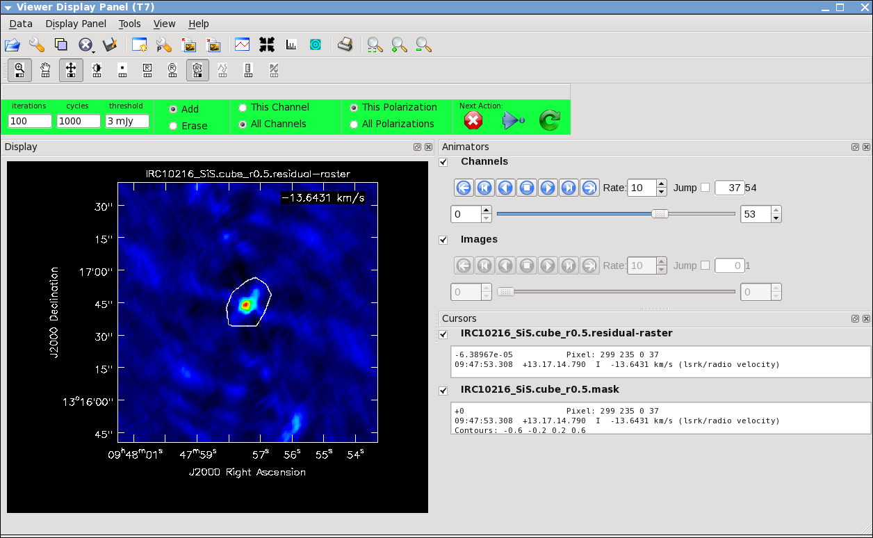
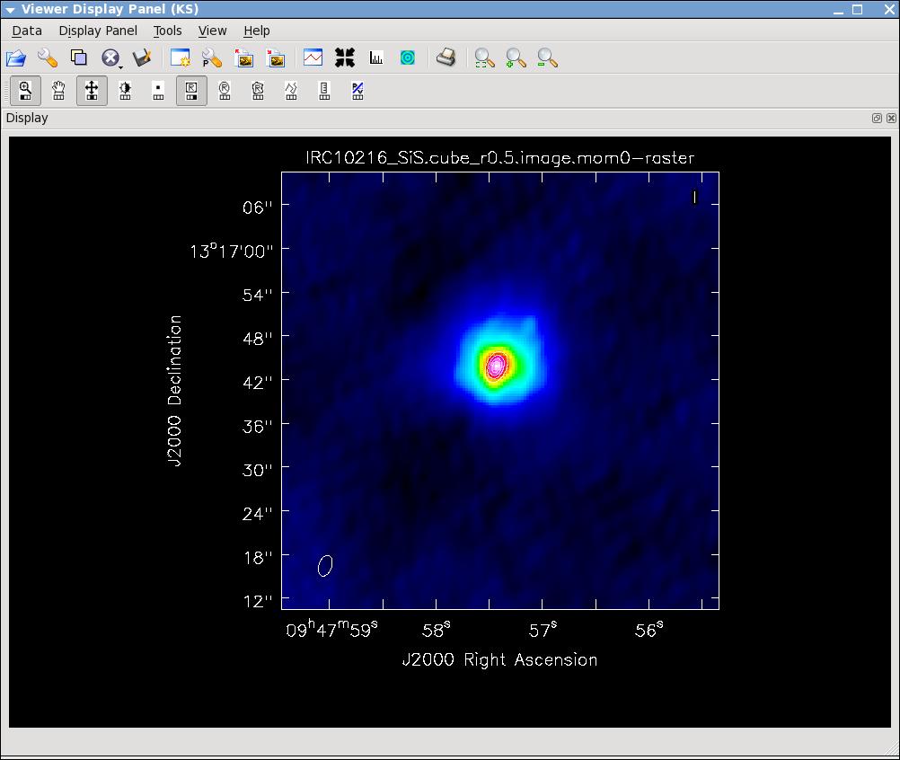
Repeat the process for the SiS line using the call below (see Figure 28). Note the emission for this line is less extended than the HC3N—this has to do with the different excitation requirements of the two different lines. The SiS is excited closer to the central star than the HC3N.
# In CASA
clean(vis='IRC10216.contsub',imagename='IRC10216_SiS.cube_r0.5',
      imagermode='csclean',
      imsize=300,cell=['0.4arcsec'],spw='1:5~58',
      mode='velocity',interpolation='linear',
      restfreq='36.30963GHz',outframe='LSRK',
      weighting='briggs',robust=0.5,
      interactive=T,
      threshold='3.0mJy',niter=100000)
You can look at both cubes using the viewer, and use the tape deck controls to play the cube as a movie.
# In CASA
viewer
Image the Continuum data
Below the use of parameter mode='mfs' will make a single multi-frequency synthesis image out of the specified spw/channels. Again, you should make an interactive clean mask. Since no threshold is set, you will need to stop cleaning when the residual looks noise like using the red X Next Action button ![]() (it will be done when the viewer comes back the second time). The continuum for IRC10216 is very weak but interesting—it is essentially tracing the photosphere of the AGB star.
(it will be done when the viewer comes back the second time). The continuum for IRC10216 is very weak but interesting—it is essentially tracing the photosphere of the AGB star.
The continuum data set produced with parameter wantcont=True in uvcontsub2 is the model fit. To image the continuum itself, use the line-free channels.
# In CASA
clean(vis='IRC10216',imagename='IRC10216.36GHzcont',
      mode='mfs',imagermode='csclean',
      imsize=300,cell=['0.4arcsec'],spw='0~1:5~14,0~1:48~59',
      weighting='briggs',robust=0.5,
      interactive=T)
Now look at the result in the viewer, if you like:
# In CASA
viewer
Image Analysis and Viewing
Next, make integrated intensity maps (moment 0) and intensity-weighted velocity maps (moment 1). For HC3N, we also produce a velocity dispersion, peak flux, and median map. All are derived with immoments. In order to do this, we'll want to know what channels the line emission starts and ends on and the rms noise in a single channel. First open with the viewer file IRC10216_HC3N.cube_r0.5.image:
# In CASA
viewer('IRC10216_HC3N.cube_r0.5.image')
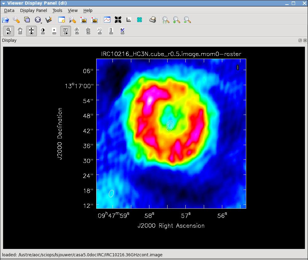
Use the tape deck controls to see which channels have significant line emission. For HC3N, the line channel range in the cube is 10 to 39, which is 16 to 45 in the original 64-channel uv-data, but for imaging the 5 beginning and ending channels were discarded by selecting 0:5~58, which resulted in a 54 channel image cube (see Figure 29); this is also the same for SiS (see Figure 30).
Then use the tape deck to go to a line free channel, select the box region tool and make a box. When you double click in the box, the image statistics for the channel you are on will print to the terminal. Move the box around a bit to see what the variation in rms noise is. You should get something like 2 mJy. Note that the rms is much worse in channels with strong emission because of the low dynamic range of these data. If you want the box tool to go away, i.e., if you want to make a new one, press the Escape key.
Now let's make the moment 0 and moment 1 maps. For moment 0, it's best to limit the calculation to image channels with significant signal in them, but not to apply a flux cutoff, as this will bias the derived integrated intensities upward.
# In CASA
immoments(imagename='IRC10216_HC3N.cube_r0.5.image',moments=[0],
          axis='spectral',
          chans='10~39',
          outfile='IRC10216_HC3N.cube_r0.5.image.mom0')
# In CASA
immoments(imagename='IRC10216_SiS.cube_r0.5.image',moments=[0],
          axis='spectral',
          chans='10~39',
          outfile='IRC10216_SiS.cube_r0.5.image.mom0')
To have a look at these, use the viewer (see Figures 29 & 30):
# In CASA
viewer('IRC10216_HC3N.cube_r0.5.image.mom0')
#
viewer('IRC10216_SiS.cube_r0.5.image.mom0')
For moment 1, it is essential to apply a conservative flux cutoff to limit the calculation to high signal-to-noise areas. Here we use about 5σ:
# In CASA
immoments(imagename='IRC10216_HC3N.cube_r0.5.image',moments=[1],
          axis='spectral',
          chans='10~39',excludepix=[-100,0.01],
          outfile='IRC10216_HC3N.cube_r0.5.image.mom1')
# In CASA
immoments(imagename='IRC10216_SiS.cube_r0.5.image',moments=[1],
          axis='spectral',
          chans='10~39',excludepix=[-100,0.01],
          outfile='IRC10216_SiS.cube_r0.5.image.mom1')
Finally, we will do velocity dispersion, peak flux, and median map in a single step for HC3N. Task immoments can perform these steps even though the latter two are not moments in a mathematical sense. Check the help file to find out the options. Peak flux and median are produced with the moment parameter set to 8 and 3:
# In CASA
immoments(imagename='IRC10216_HC3N.cube_r0.5.image',moments=[2,8,3],
          axis='spectral',
          chans='10~39',excludepix=[-100,0.01],
          outfile='IRC10216_HC3N.cube_r0.5.image.extramoms')
will create the files IRC10216_HC3N.cube_r0.5.image.extramoms.weighted_dispersion_coord, IRC10216_HC3N.cube_r0.5.image.extramoms.median, and IRC10216_HC3N.cube_r0.5.image.extramoms.maximum.
Now use the viewer to further explore the images you've made.
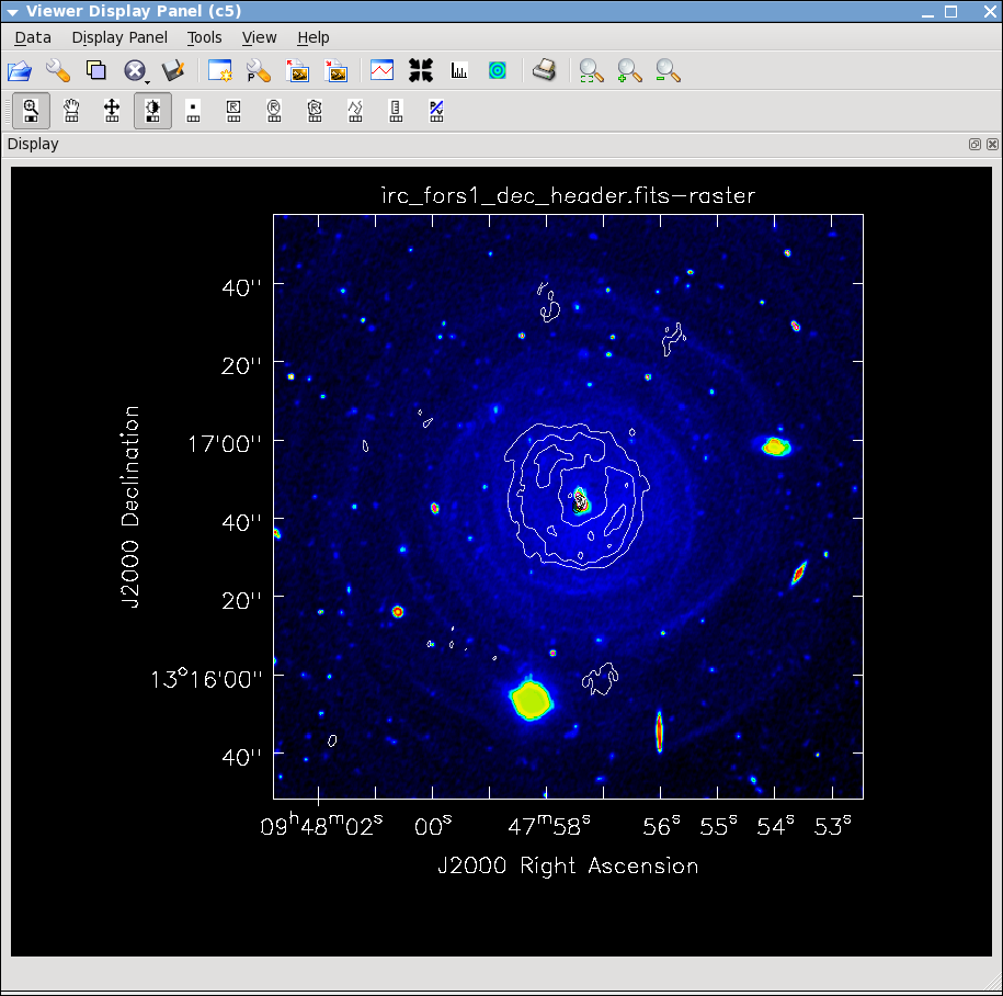
For fun you can download the VLT V-band image at http://casa.nrao.edu/Data/EVLA/IRC10216/irc_fors1_dec_header.fits kindly provided by Izan Leão and overlay the moment images and 36 GHz continuum (see Figure 31). More information about the dust properties can be found in the Leão et al. (2006) paper http://adsabs.harvard.edu/abs/2006A%26A...455..187L.
The creation of position velocity cuts from the viewer is currently being developed and hopefully available soon in CASA. If you are interested in a work-around, you may have a look at the pV casaguide. Masking the data cube to extract the emission is described in the Masking_images_for_analysis page.
Spectrum Fitting
Frequently, one may like to fit Gaussians or polynomials to the spectral line in the data cube. This can be done with CASA's specfit task; specfit can fit those functions to an average spectrum defined by some bounding box, or, alternatively, for each pixel. We will perform the fitting an average spectrum.
Fitting an average spectrum
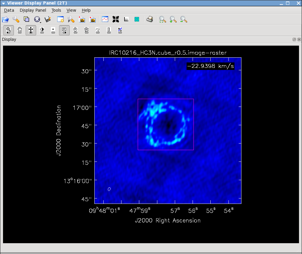
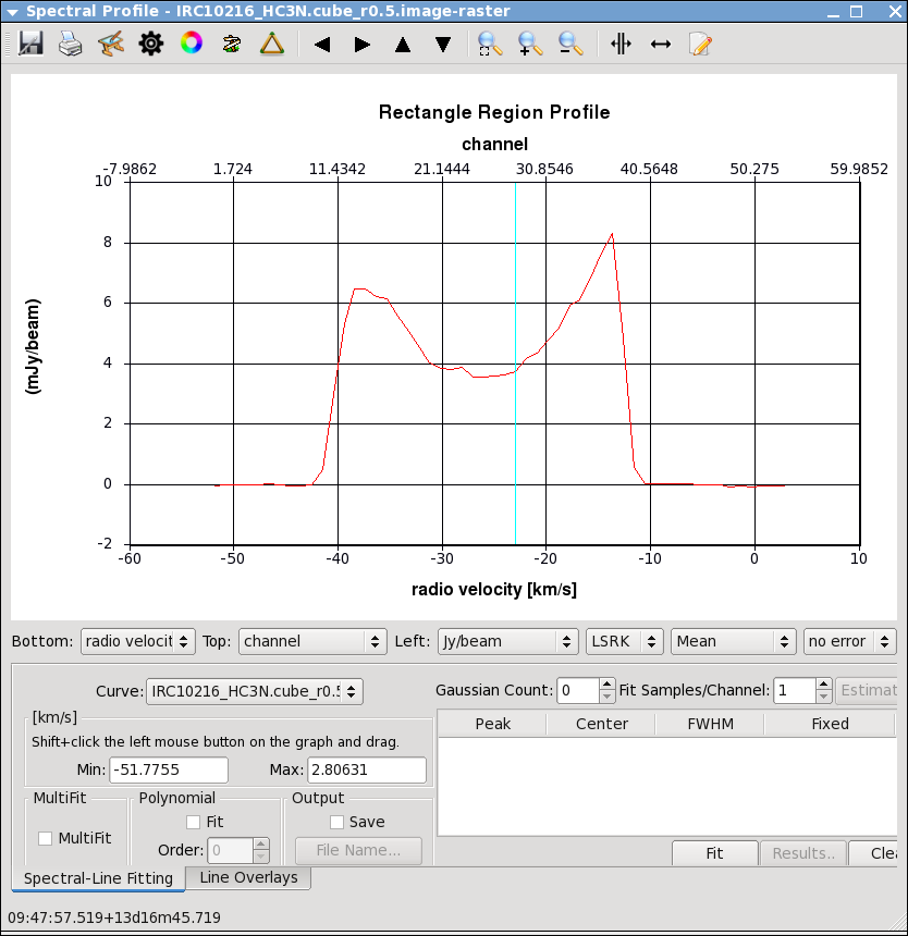
First, we want to inspect the spectrum. Load the image into the viewer (here the HC3N image cube), select spectral profile from the Tools menu and open a region with the mouse button that is assigned to the rectangular R region in the tool bar. Best to do this at a plane that shows the entire extent of the source. The average spectrum will be displayed in a separate panel (see Figure 32).
To fit this profile in specfit, we need a region file outlining the 2-D region that is averaged (the green box in the viewer screenshot). In the following we use the new CASA region format (CASA 3.3 and higher) that is described at the CASA Region Format page. Following the guidelines on that page, we create a file named specfit.crtf that describes a box with its [[x1,y1],[x2,y2]] corners in J2000 RA DEC coordinates. Use any text editor (e.g., emacs, vi, etc.) to create the file specfit.crtf with the following box parameters:
#CRTFv0
box[[09:47:59.2, 13.16.24], [09:47:55.8, 13.17.09]]
We will fit two Gaussians to the two peaks of the spectrum (the scientific merit is debatable). A file with initial values for the fit can be provided via the parapmeter estimates—see specfit for more information. Here we will let CASA figure out the start values by itself:
# In CASA
myfit = specfit(imagename='IRC10216_HC3N.cube_r0.5.image', region='specfit.crtf', multifit=F,
        estimates='', ngauss=2)
Note that the output is stored in a Python dictionary called "myfit", as well as printed to the CASA logger. You should get something similar to the following output, the results will vary based on your cleaning regions, depths, etc.:
Results for component 0:
    Type     : GAUSSIAN
    Peak     : 5.58 +/- 0.42 mJy/beam
    Center   : -16.87 +/- 0.40 km/s
               33.89 +/- 0.39 pixel
    FWHM     : 9.50 +/- 0.97 km/s
               9.22 +/- 0.94 pixel
    Integral : 56.5 +/- 7.2 mJy/beam.km/s
Results for component 1:
    Type     : GAUSSIAN
    Peak     : 4.85 +/- 0.36 mJy/beam
    Center   : -33.93 +/- 0.53 km/s
               17.33 +/- 0.52 pixel
    FWHM     : 13.2 +/- 1.4 km/s
               12.8 +/- 1.3 pixel
    Integral : 68.2 +/- 8.8 mJy/beam.km/s
which seems to have caught the two peaks pretty well.
Self-Calibration
The many different aspects of self-calibration could fill several casaguides. Here we describe a simple process for this particular relatively low S/N data (low S/N per channel, at least).
While running clean above, the model column for each channel will have been filled with the clean model (if you made a Fourier transform of this model, you would see an image of the clean components).
We choose to do the self cal on the spw=1 SiS line data because it has the strongest emission in a single channel and is a bit more compact than the HC3N data. We will run gaincal specifying the channel in the uv-data that has the brightest peak in the image (use the viewer to figure out which channel this is for spw=1), note the peak flux. Since we started the image with a channel range, we need to account for the fact that the image channel numbers do not map exactly to the uv-data channel numbers (they are off by 5 so that channel 13 in the image is roughly channel 19 in the uv-data).
Next we need to understand the S/N of the data. In particular, to self-cal, you need enough signal on a single baseline over the course of your chosen solint to get a S/N of about 3. We calculated above an average rms noise of about 2 mJy/beam/channel for the entire timerange (about 95 minutes of on-source time) and all antennas (16). We can use our knowledge of the radiometer equation (see VLA Sensitivity) where rms scales as 1/sqrt(time * #baselines), and the number of baselines= N(N-1)/2 and N=# of antennas. So the rms noise on one baseline, for one 10 second integration in this observation is given by:
[math]\displaystyle{ {\rm RMS(baseline)} = {\rm 2\ mJy\ beam^{-1}\ channel^{-1}} \sqrt{ \frac{95\times 60\ {\rm sec}}{10\ {\rm sec}}\times\frac{16\times 15}{2\times 1}}\ {\sim}\ 500\ {\rm mJy\ beam^{-1}\ channel^{-1}} }[/math]
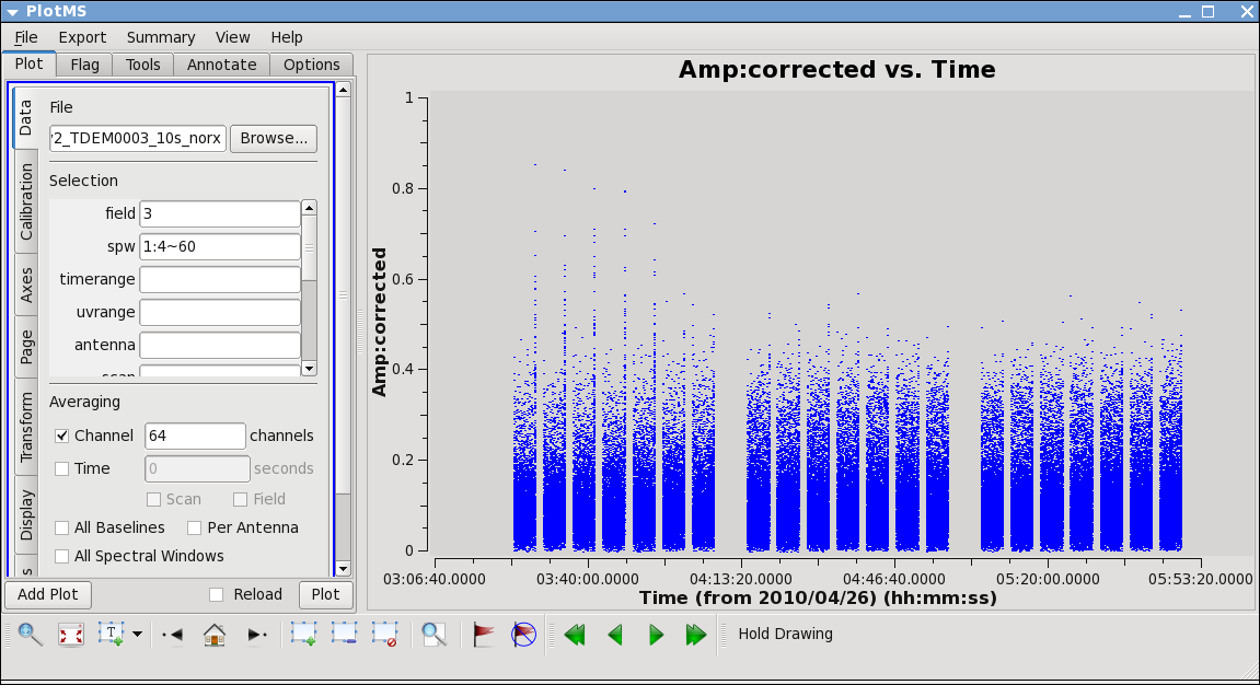
The 95 minutes of on-source time can be estimated from a plot where you can sum up the amount of time on a source (see Figure 34):
# In CASA
plotms(vis='day2_TDEM0003_10s_norx',field='3',ydatacolumn='corrected',
       xaxis='time',yaxis='amp',correlation='RR,LL',
       avgchannel='64',spw='1:4~60',antenna='')
This analysis suggests that the rms noise on one baseline, for one 10 second integration, is only about 500 mJy. In contrast, the peak flux density in the strongest SiS channel is only about 200 mJy (you can check using the viewer). Since the emission is fairly compact, most baselines will see about this peak flux; this is why we choose the more compact of the two possible lines. Thus, a 10 second solution interval is not enough to get a SNR of at least 3 on a 200 mJy peak. We need to use a solint large enough so that the rms noise is not worse than about 1/3 of 200 mJy. Thus, a solint of 10 minutes is about the shortest we can use and be reasonably confident of the solutions.
Now we run gaincal with the solint we have determined. Note that because our desired solint is more than the scan time, we need to include parameter combine='scan' .
# In CASA
gaincal(vis='IRC10216',caltable='pcal_ch19one_10min',
        spw='1:19',calmode='p',solint='10min',combine='scan',
        refant='ea02',minsnr=3.0)
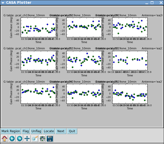
Next, look at the solutions:
# In CASA
plotcal(caltable='pcal_ch19one_10min',xaxis='time',yaxis='phase',
        iteration='antenna',subplot=331,plotrange=[0,0,-50,50])
For some antennas you can see clear global trends away from zero: ea08, ea21, and ea24 are examples, and you can also see some smaller variations with time (see Figure 35).
Now explore whether applying this solution actually improves matters. To do this, run applycal to apply the solutions to the line dataset for both spw. Use parameter spwmap to tell it that the solutions derived for spw=1 should be applied to both spw=0 and spw=1. Again, it's important to set parameter calwt=F here.
# In CASA
applycal(vis='IRC10216.contsub',field='',spw='0,1',
        gaintable=['pcal_ch19one_10min'],spwmap=[[1,1]],calwt=F)
Note: in this example we ran the self-cal steps on the full uv continuum subtracted spectral line data set. For a more complex iterative self-calibration procedure, you may find it easier to split off the channel/spw you want to experiment on with split, and then do all the imaging (clean) and gaincal steps with it. The gaincal tables created on the single channel can still be applied with applycal to the multi-channel/spw dataset. If you do this, keep in mind that once split, the single-channel data will have its spw ID reset to 0 (you can check with listobs), no matter what spw it came from. Thus, in order to applycal with it, you would need parameter spwmap=[[0,0]].
To save time, use the clean mask you made before and run in a non-interactive mode. You can use a mask over again as long as the number of channels in the clean call haven't changed. You can change cell or imsize and it will still do the right thing.
# In CASA
clean(vis='IRC10216.contsub',imagename='IRC10216_HC3N.cube_r0.5.pselfcal',
      imagermode='csclean',
      imsize=300,cell=['0.4arcsec'],spw='0:5~58',
      mode='velocity',interpolation='linear',
      restfreq='36.39232GHz',outframe='LSRK',
      weighting='briggs',robust=0.5,
      mask='IRC10216_HC3N.cube_r0.5.mask',
      interactive=F,threshold='3.0mJy',niter=100000)
# In CASA
clean(vis='IRC10216.contsub',imagename='IRC10216_SiS.cube_r0.5.pselfcal',
      imagermode='csclean',
      imsize=300,cell=['0.4arcsec'],spw='1:5~58',
      mode='velocity',interpolation='linear',
      restfreq='36.30963GHz',outframe='LSRK',
      weighting='briggs',robust=0.5,
      mask='IRC10216_SiS.cube_r0.5.mask',
      interactive=F,threshold='3.0mJy',niter=100000)
Now investigate the original and self-calibrated images in the viewer. You will find that even this single self-cal step significantly improves the images. Try opening both versions of the SiS image cubes. Select a bright channel via the tape deck controls, then use the wrench and pwrench tools to make a plot setting the same image range for both cubes, and two panels in x, then to see both images of that channel side-by-side click the blink toggle (see Figure 36 for more tips on setup parameters).
Figure 36: Original and self-cal SiS images for channel 37/54, notice the decrease in residuals.
Repeat for HC3N (see Figure 37):
Figure 37: Original and self-cal HC3N images for channel 34/54, notice the decrease in residuals.
Now you can redo the moment images with the improved cubes. Be sure to change the output file names.
Questions about this tutorial? Please contact the NRAO Helpdesk.
Last checked on CASA Version 4.5.2
